squire

squire enables users to simulate models of SARS-CoV-2 epidemics. This is done using an age-structured SEIR model that also explicitly considers healthcare capacity and disease severity.

Overview

squire is a package enabling users to quickly and easily generate calibrated estimates of SARS-CoV-2 epidemic trajectories under different control scenarios. It consists of the following:

• An age-structured SEIR model incorporating explicit passage through healthcare settings and explicit progression through disease severity stages.
• The ability to calibrate the model to different epidemic start-dates based on available death data.
• Simulate the impacts of different control interventions (including general social distancing, specific shielding of elderly populations, and more stringent suppression strategies).

If you are new to squire, the best place to start is below, where we detail how to install the package, how to set up the model, and how to run it with and without control interventions.

Model Structure

Overall Structure

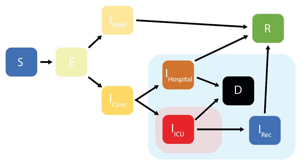
squire uses an age-structured SEIR model, with the infectious class divided into different stages reflecting progression through different disese severity pathways. These compartments are:
* S = Susceptibles
* E = Exposed (Latent Infection)
* I_Mild = Mild Infections (Not Requiring Hospitalisation)
* I_Case = Infections Requiring Hospitalisation
* I_Hospital = Hospitalised (Requires Hospital Bed)
* I_ICU = ICU (Requires ICU Bed)
* I_Rec = Recovering from ICU Stay (Requires Hospital Bed)
* R = Recovered
* D = Dead

Decision Trees for Healthcare Capacity

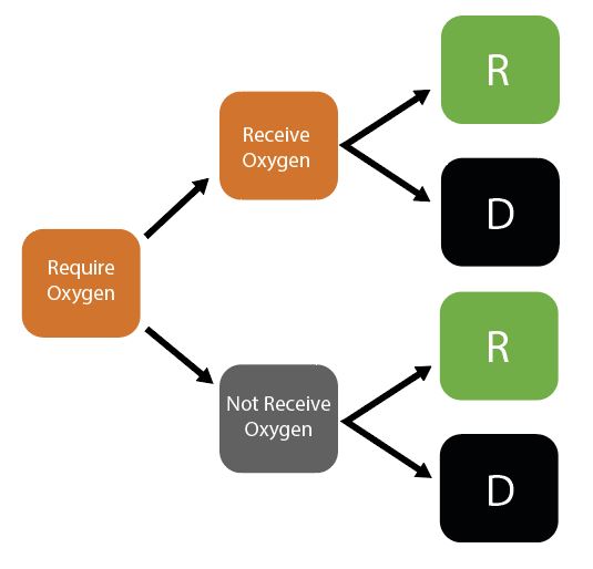
Given initial inputs of hospital/ICU bed capacity and the average time cases spend in hospital, the model dynamically tracks available hospital and ICU beds over time.

Individuals newly requiring hospitalisation (either a hospital or ICU bed) are then assigned to either receive care (if the relevant bed is available) or not (if maximum capacity would be exceeded otherwise). Whether or not an individual receives the required care modifies their probability of dying.

Installation

squire utilises the package ODIN to generate the model. ODIN implements a high-level language for implementing mathematical models and can be installed by running the following command:

install.packages("odin")

The model generated using ODIN is written in C and so you will require a compiler to install dependencies for the package and to build any models with ODIN. Windows users should install Rtools. See the relevant section in R-admin for advice. Be sure to select the “edit PATH” checkbox during installation or the tools will not be found.

The function odin::can_compile() will check if it is able to compile things, but by the time you install the package that will probably have been satisfied.

After installation of ODIN, ensure you have the devtools package installed by running the following:

install.packages("devtools")

Then install the squire package directly from GitHub by running:

devtools::install_github("mrc-ide/squire")

If you have any problems installing then please raise an issue on the squire GitHub.

If everything has installed correctly, we then need to load the package:

library(squire)

Getting Started

Running the Model (Unmitigated)

1. Running the model using baseline parameters and no control interventions

The full model is referred to as the explicit_SEEIR model, with hospital pathways explicltly exploring whether individuals will require a general hospital bed providing oxygen or an ICU bed that provides ventilation.

To run the model we need to provide at least one of the following arguments:

• country
• population and contact_matrix_set

If the country is provided, the population and contact_matrix_set will be generated (if not also specified) using the demographics and matrices specified in the global report.

To run the model by providing the country we use run_explicit_SEEIR_model():

r <- run_explicit_SEEIR_model(country = "Afghanistan")

The returned object is a squire_simulation object, which is a list of two ojects:

• output - model output
• parameters - model parameters

squire_simulation objects can be plotted as follows:

plot(r)

This plot will plot each of the compartments of the model output.

2. Changing parameters in the model.

The model has a number of parameters for setting the R0, demography, contact matrices, the durations of each compartment and the health care outcomes and healthcare availability. In addition, the initial state of the population can be changed as well as simulation parameters, such as the number of replicates, length of simulation and the timestep. For a full list of model inputs, please see the function documentation

For example, changing the initial R0 (default = 3), number of replicates ( default = 10), simualtion length (default = 365 days) and time step (default = 0.5 days), as well as setting the population and contact matrix manually:

# Get the population
pop <- get_population("United Kingdom")
population <- pop$n

# Get the mixing matrix
contact_matrix <- get_mixing_matrix("United Kingdom")

# run the model
r <- run_explicit_SEEIR_model(population = population, 
                              contact_matrix_set = contact_matrix,
                              R0 = 2.5, 
                              time_period = 200,
                              dt = 1,
                              replicates = 5)
plot(r)

We can also change the R0 and contact matrix at set time points, to reflect changing behaviour resulting from interventions. For example to set a 80% reduction in the contact matrix after 50 days :

# run the model
r <- run_explicit_SEEIR_model(population = population, 
                              tt_contact_matrix = c(0, 50),
                              contact_matrix_set = list(contact_matrix,
                                                        contact_matrix*0.2),
                              R0 = 2.5, 
                              time_period = 200,
                              dt = 1,
                              replicates = 5)
plot(r)

To show an 80% reduction after 50 days but only maintained for 30 days :

# run the model
r <- run_explicit_SEEIR_model(population = population, 
                              tt_contact_matrix = c(0, 50, 80),
                              contact_matrix_set = list(contact_matrix,
                                                        contact_matrix*0.2,
                                                        contact_matrix),
                              R0 = 2.5, 
                              time_period = 200,
                              dt = 1,
                              replicates = 5)
plot(r)

Alternatively, we could set a changing R0, which falls below 1 after 50 days:

# run the model
r <- run_explicit_SEEIR_model(population = population, 
                              contact_matrix_set = contact_matrix,
                              tt_R0 = c(0, 50),
                              R0 = c(2.5, 0.9),
                              time_period = 200,
                              dt = 1,
                              replicates = 5)
plot(r)

3. Extracting and Plotting Relevant Outputs

Alternative summaries of the models can be created, which give commonly reported measures, such as deaths, number of ICU beds and general hospital beds required.

These could be created by using the outputs seen in the previous section, e.g. r$output$ICase1 + r$output$ICase2 to get the total symptomatic cases.

However, accessing outputs this waus is much slower. A quicker way is to change the simulation output with output_transform = FALSE, which will not transform the outputs produced by odin.

# run the model
r <- run_explicit_SEEIR_model(country = "Afghanistan",
                              output_transform = FALSE)

To access the outputs we can use untransformed_output, specifying
which compartments are to be returned, and which specific summary outputs related to case incidence, death incidence and hospital bed demands are needed:

gcu <- untransformed_output(r, compartments = c("S", "R"),
                               deaths = TRUE, 
                               cases = TRUE, 
                               beds = TRUE)

This object can then be easily plotted:

plot(gcu)

4. Calibrating the Model to Observed Deaths Data

The model can be simply calibrated to time series of deaths reported in settings. This can be conducted using the calibrate function, by providing a data frame of date and deaths. For example:

# create dummy data
df <- data.frame("date" = Sys.Date() - 0:6,
                 "deaths" = c(6, 2, 1, 1, 0, 0, 0),
                 "cases" = c(394, 101, 89, 4, 0, 0, 0))
df
#>         date deaths cases
#> 1 2020-04-10      6   394
#> 2 2020-04-09      2   101
#> 3 2020-04-08      1    89
#> 4 2020-04-07      1     4
#> 5 2020-04-06      0     0
#> 6 2020-04-05      0     0
#> 7 2020-04-04      0     0

# run calibrate
out <- calibrate(data = df, country = "Senegal", replicates = 10)

Simulation replicates are aligned to the current death total and the outputs are returned as a squire_calibration object, which has dedicated plotting functions.

These allow the predicted cumulative cases based from the observed deaths to be plotted:

plot(out, what = "cases")

Additionally, we can plot the incidence of deaths as well as the healthcare demands:

plot(out, what = "healthcare")
#> Warning: Removed 3315 row(s) containing missing values (geom_path).
#> Warning: Removed 351 row(s) containing missing values (geom_path).

We can also control how far we forecast. To forecast for 14 days:

plot(out, what = "healthcare", forecast = 14)
#> Warning: Removed 3315 row(s) containing missing values (geom_path).
#> Warning: Removed 351 row(s) containing missing values (geom_path).