There was a nice paper out this week on Lassa Fever virus (LASV) in Cell by Pardis Sabeti and colleagues. They very laudibly included all of the supplementary files, including sequence data, sampling dates, etc., so I thought I would take a quick look to see what sort of signal was in the data. The data was collected over the course of five years, so such exploratory analyses can't really do justice to the data, nor to the effort in collecting it, but my intention is to show how one can get an idea of the phylodynamics, and some of the issues with the data, with relatively little effort.
The first thing we need is a tree. Rather than obtain a sample of trees (via a Bayesian approach or a bootstrap), I will generate a maximum likelihood tree quickly with ExaML. First, we need to convert the multiple sequence file (in PHYLIP format) to a binary format. I'm using non-identical sequences of the L segment of LASV sampled from Sierra Leone in Phylip sequential format, named LASV.phy, where the sequence names end with a hyphen and the sampling year. This is important, as we will extract the sampling times from the sequences later.
parse-examl -s LASV.phy -m DNA -n LASVThis leaves around a RAxML_info file that we don't need, so we remove that as well.
rm RAxML_info.LASVThis will generate a file LASV.binary that we can pass to ExaML. We also need to generate a starting tree for ExaML using (e.g.) RAxML, using -y to return a parsimony tree.
raxmlHPC-PTHREADS-SSE3 -y -m GTRCAT -p 12345 -s LASV.phy -n LASVIn order to get a tree faster, the convergence criterion can based on relative Robinson-Foulds distance (-D), rather than basing convergence on the likelihood. The following fits a position-specific rate (-m PSR) model with 25 (-c 25) categories, keeping 10 trees (-B 10).
examl -a -B 10 -c 25 -D -m PSR -n LASV -s LASV.binary -t RAxML_parsimonyTree.LASVExaML leaves around a bunch of checkpoint files, so let's get rid of those.
rm ExaML_binaryCheckpoint.*In order to get a time-stamped phylogeny, we will also need a table of tip dates, which we can extract from the sequence names using this R snippet.
library(ape)
library(magrittr)

lasv <- read.dna("LASV.phy",format="sequential")
lasv.tipnames <- row.names(lasv)
lasv.tipdates <- lasv.tipnames %>% strsplit(.,"-",fixed=TRUE) %>% lapply(.,tail,1) %>% unlist %>% as.double
lasv.df <- data.frame(c(length(lasv.tipnames),lasv.tipnames),c("",lasv.tipdates))
write.table(lasv.df,"LASV.tipdates",col.names=FALSE,row.names=FALSE,quote=FALSE,sep="\t")
Fast methods don't work well for low-diversity sequences, so we resolve multifurcations, and make sure we don't have any zero branch lengths.
library(ape)

lasv.tree <- read.tree("ExaML_result.LASV")
lasv.tree <- unroot(lasv.tree)
lasv.tree.binary <- multi2di(lasv.tree)
lasv.tree.binary$edge.length <- lasv.tree.binary$edge.length+1e-6
write.tree(lasv.tree.binary,"LASV.nwk")
We can use this tree to get an idea of evolutionary rates and time to the most recent common ancestor. For example, using root-to-tip regression (an idea implemented in Path-O-Gen by Andrew Rambaut, as well as the rtt function by Rosemary McCloskey and Emmanuel Paradis in the R library ape)
./rtt.R LASV.nwk LASV_rttThis generates a TMRCA and evolutionary rate as follows.
| TMRCA | SubstRate |
|---|---|
| 1889 | 0.00138 |
We can also take the rooted tree from rtt and estimate the evolutionary rate using TREBLE (the C code in treble.R is written by Jack O'Brien, which is linked to R with the wonderful inline library).
./treble.R LASV_rtt.tre LASV_trebleThis gives a rather different answer for the TMRCA; this suggests that we may have to take the results above with a pinch of salt.
| TMRCA | SubstRate |
|---|---|
| 1794 | 0.001097 |
One of the fastest methods to obtain clock-like trees is least-squares dating, as implemented in LSD. However, it doesn't work well for low-diversity sequences (and often segfaults). Instead, I use a modified version of chronos, which roots the tree and estimates a TMRCA using root to tip regression, then fits a clock with discrete rate classes, increasing the number of rate classes until there is no improvement in PHIIC, an information criterion developed with molecular clocks in mind by Emmanuel Paradis. The tweaks to the implementation in R are mainly due to Rosemary McCloskey (again), with a few minor ones by myself.
./chronos.R LASV.nwk LASV_chronosAlthough this appears to favour a strict clock, the fact that a two-rate clock has a worse likelihood shows that there are convergence issues. Still, let's carry on with looking at the 'clockified' tree. I'll display it using some code hacked from some ggplot2 magic from Anton Camacho ( @ntncmch ), code that ultimately made it into Thibaut Jombart's ( @thibautjombart ) OutbreakTools package.
library(ape)
library(magrittr)
library(ggplot2)
library(scales)
source("phylo2ggphy.R")
source("plot_ggphy.R")
lasv.chronos <- read.tree("LASV_chronos.nwk")
lasv.chronos <- ladderize(lasv.chronos)
lasv.host <- rep("Human",length(lasv.chronos$tip.label))
lasv.host[grep("Josiah",lasv.chronos$tip.label)] <- "Lab"
lasv.host[grep("LM",lasv.chronos$tip.label)] <- "Mastomys"
lasv.host[grep("ZO",lasv.chronos$tip.label)] <- "Mastomys"
lasv.annotations <- data.frame(taxa=lasv.chronos$tip.label,Host=lasv.host)
lasv.tipdates <- strsplit(lasv.chronos$tip.label,"-",fixed=TRUE) %>% lapply(.,tail,1) %>% unlist %>% as.double
lasv.tipdates <- as.Date(paste(lasv.tipdates,"-01-01",sep=""))
lasv.ggphy <- phylo2ggphy(lasv.chronos,tip_dates=lasv.tipdates,branch_unit="year")
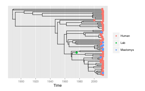
plot_ggphy(lasv.ggphy,tip_labels=F,tip_attribute=lasv.annotations,var_tip_labels="taxa",var_tip_colour="Host")This demonstrates the intermingling of human and rodent sequences expected under multiple cross-species transmissions.
Lastly, but not least, we can look at a skyline plot, generated using an approach developed by Julia Palacios and Vladimir Minin, which uses integrated nested Laplace approximation (INLA).
library(ape)
library(INLA)
library(magrittr)
library(ggplot2)
source("skyride.R")

lasv.chronos <- read.tree("LASV_chronos.nwk")
lasv.sr <- calculate.heterochronous.skyride(lasv.chronos)
lasv.tipdates <- strsplit(lasv.chronos$tip.label,"-",fixed=TRUE) %>% lapply(.,tail,1) %>% unlist %>% as.double
lasv.sr$year <- max(lasv.tipdates)-lasv.sr$time
ggplot(data=lasv.sr,aes(x=year))+geom_line(aes(y=sr.median))+ylab(expression(N[e]))+xlab("Time since present")+scale_y_log10(limits=c(10,1000))+theme(strip.text.x=element_text(size = rel(0.6)))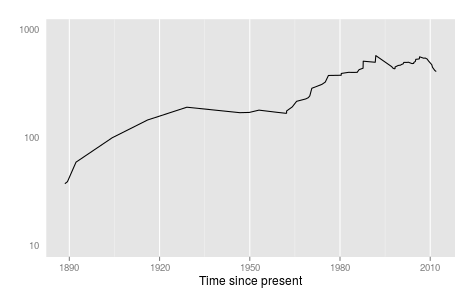
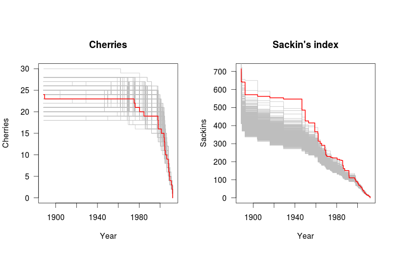
Last (for now), but not least, a simple test for asymmetry (above and beyond what one would expect from a coalescent process) devised by Bethany Dearlove, and recently published by us, and available on GitHub. This compares measures of tree shape with that expected under permuted trees with the same sampling and coalescence times. Below, I compute 'cherries', the number of adjacent tips on the tree (lower=more asymmetry) and Sackin's index (higher=more asymmetry).
library(ape)
library(magrittr)
library(treeImbalance)

lasv.chronos <- read.tree("LASV_chronos.nwk")
lasv.tipdates <- strsplit(lasv.chronos$tip.label,"-",fixed=TRUE) %>% lapply(.,tail,1) %>% unlist %>% as.double

lasv.cherries.obs <- ct(lasv.chronos)
lasv.sackins.obs <- snt(lasv.chronos)

treelist <- list()
nsims <- 1000
for(i in 1:nsims){
  treelist[[i]] <- getSimTree(lasv.chronos)
}

lasv.cherries.sim <- lapply(treelist,ct)
lasv.sackins.sim <- lapply(treelist,snt)

par(mfrow=c(1,2),pty="s")
plot(max(lasv.tipdates)-lasv.cherries.obs[[1]],lasv.cherries.obs[[2]],col="red",xlab="Year",ylab="Cherries",las=1,ylim=c(0,30),type="n",main="Cherries")
for(i in 1:nsims){
  lines(max(lasv.tipdates)-lasv.cherries.sim[[i]][[1]],lasv.cherries.sim[[i]][[2]],type="s",col="gray")
}
lines(max(lasv.tipdates)-lasv.cherries.obs[[1]],lasv.cherries.obs[[2]],type="s",col="red",lwd=2)
plot(max(lasv.tipdates)-lasv.sackins.obs[[1]],lasv.sackins.obs[[2]],col="red",xlab="Year",ylab="Sackins",las=1,type="n",main="Sackin's index")
for(i in 1:nsims){
  lines(max(lasv.tipdates)-lasv.sackins.sim[[i]][[1]],lasv.sackins.sim[[i]][[2]],type="s",col="gray")
}
lines(max(lasv.tipdates)-lasv.sackins.obs[[1]],lasv.sackins.obs[[2]],type="s",col="red",lwd=2)
This shows that the phylogeny is rather imbalanced (according to Sackin's index) compared to what one would expect from a homogenous population.
Running these analyses took far less time than that taken to write this README, hopefully encouraging others to conduct exploratory phylodynamic analysis before launching into a full-blown BEAST run.