ProtSpace3D

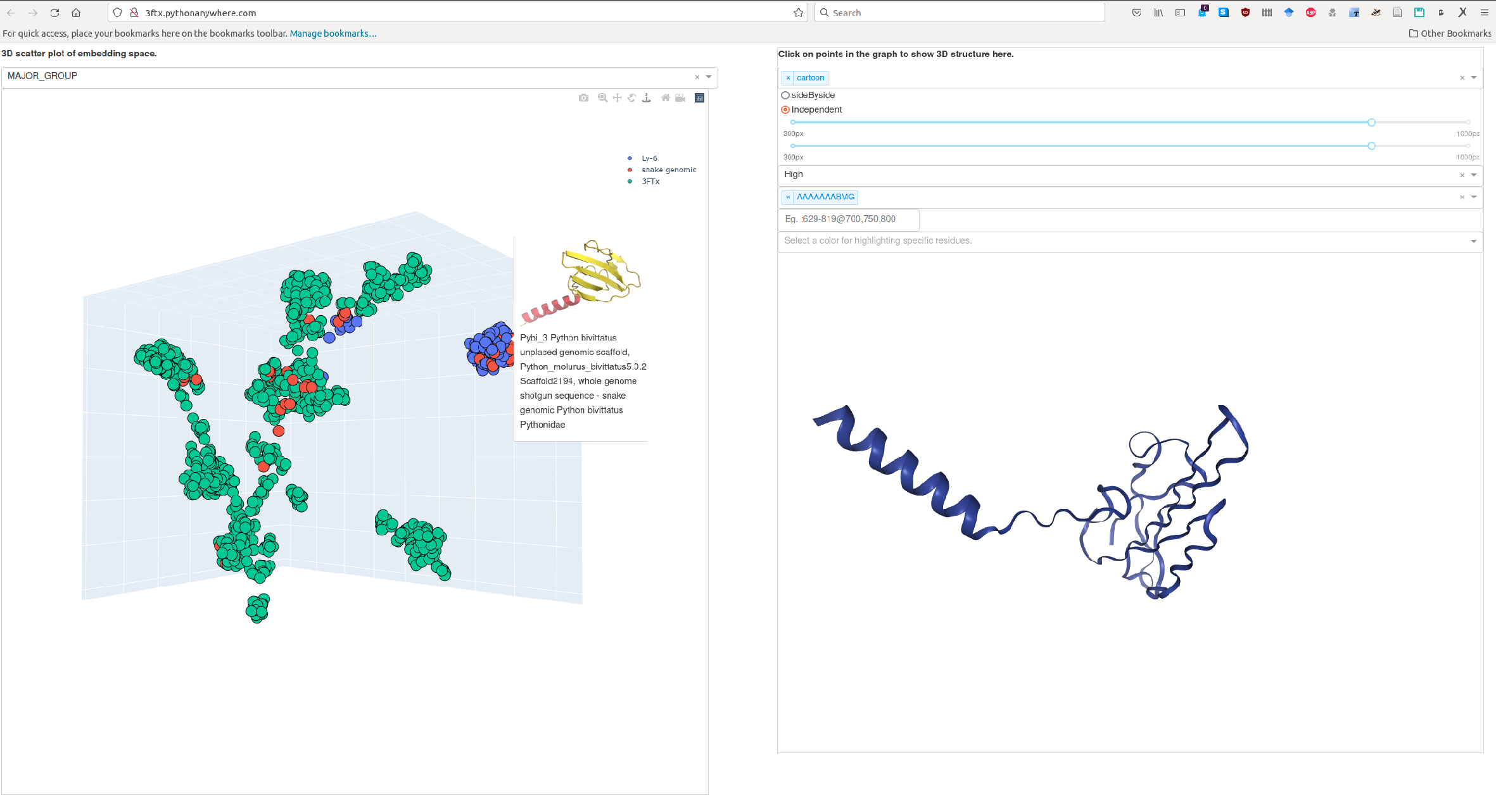
This repository holds example code on how to visualize a set of proteins in 3D space. Proteins are first represented as high-dimensional vector representations (embeddings) derived from protein language models (pLMs) which are later projected to 3D for further analysis. When hovering over points (each point is a protein), images of 3D structures predicted via ColabFold/AlphaFold2 (AF2) are shown. An interactive 3D visualization of the same structure can be shown in the right panel by clicking on one of the points/proteins. There are various options for visualizing a structure. Instead of clicking on a point/protein, you can also search for its ID in the search-field in the right panel.

Using the family of Three-finger toxins (3FTx), we exemplify how such analysis can help to derive hypothesis on the phylogenetics of this family. An example of this is hosted here.

Getting started

Clone this repository and get started as described in the Usage section below:

git clone https://github.com/mheinzinger/ProtSpace3D.git

Set up a local python virtual environment and install dependencies:

python3 -m venv venv
. venv/bin/activate
pip install --upgrade pip wheel
cd ProtSpace3D
pip install -r requirements.txt
wget https://rostlab.org/~deepppi/ProtSpace3D/mysite.zip
unzip -q mysite.zip

Usage

Simply run the dashboard via:

python app.py

Next, you can access the 3D visulization by accessing http://127.0.0.1:8050/ in your browser.

How to visualize a different set

In order to visualize your own dataset, you need the following files:

• A standard FASTA file holding your protein sequences
• An H5-file holding per-protein embeddings, i.e., one fixed-length vector for each protein irrespective of its length. In the example here, ProtT5 per-protein embeddings were used (1024-d) for the FASTA file. Keys are FASTA-IDs, values are embeddings. Embeddings can be computed using, e.g., Colab .
• A CSV which holds FASTA-IDs in the first field and (potentially various) class-labels for coloring protein groups in the other fields. Depending on which fields/columns you want to use to color your plot, you might need to adjust the read_csv function in app.py.

In case you only want a 3D scatter plot, you can now use the scatterExample . In this case, it's sufficient to download the folder example_input to the same directory as your scatter_example.py script. If you also want to visualize 3D structures alongside the embedding space, you'll also need the following two directories:

• A directory holding (predicted) protein 3D structures. In the example, we used ColabFold to predict protein structures. File names need to match the IDs from the FASTA (but ending on .pdb)
• A directory holding images/PNGs of the PDB files. File names need to match again the IDs (but ending on .png). PNGs can be generated using for this script. Tip: you can use mogrify -trim *.png to truncate white borders from PNGs.

What is crucial here is the mapping between the files; all files need to use the same IDs. Optimally, you start with a FASTA file that holds final IDs. From this file you generate embeddings and store them in H5 using the same IDs as keys. The CSV can be used to map between different sets of IDs and it holds the class labels which you want to color your proteins.