ThreeD_step2

2. Moving Cells

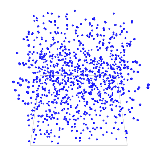
This second step model adds the moving3D skill to the cell agents and simply makes the cell agents move by defining a reflex that will call the action move. We will also add additional visual information to the display.

Formulation

• Redefining the shape of the world with a 3D Shape.
• Attaching new skills (moving3D) to cell agents.
• Modify cell aspect.
• Add a graphics layer.

Model Definition

Global Section

Global variable

We use a new global variable called environment_size to define the size of our 3D environment. In the global section, we define the new variable:

int environment_size <-100;

Then we redefine the shape of the world (by default the shape of the world is a 100x100 square) as a cube that will have the size defined by the environment_size variable. To do so we change the shape of the world in the global section:

geometry shape <- cube(environment_size);	

Model initialization

When we created the cell agents, we want to place them randomly in the 3D environment. To do so we set the location with a random value for x, y and z between 0 and environment_size.

create cell number: nb_cells { 
  location <- {rnd(environment_size), rnd(environment_size), rnd(environment_size)};       
}

Moving3D skills

In the previous example, we only created cell agents that did not have any behavior. In this step we want to make them move. To do so we add a moving3D skill to the cell species.

More information on built-in skills proposed by GAMA can be found here.

species cell skills: [moving3D]{
...  	
}

Then we define a new reflex for the species cell that consists in calling the action move bundled in moving3D skill.

reflex move {
    do move;
}	                    

Finally we modify a bit the aspect of the sphere to set its size according to the environment_size global variable previously defined.

aspect default {
    draw sphere(environment_size*0.01) color: #blue;   
}

Experiment

The experiment is the same as the previous one except that we will display the bounds of the environment by using a graphics layer.

graphics "env" {
    draw cube(environment_size) color: #black wireframe: true;	
}

Output

output {
    display View1 type:opengl{
        graphics "env"{
            draw cube(environment_size) color: #black wireframe: true;	
        }
        species cell;  
    }
}

Complete Model

https://github.com/gama-platform/gama/blob/GAMA_1.9.2/msi.gama.models/models/Tutorials/3D/models/Model%2002.gaml