flatland_railway_extension

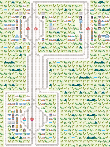
This repo extends Flatland Framework with helpful features.

Extended RailEnv

• class MultiResourcesAllocationRailEnv extends RailEnv

  MultiResourcesAllocationRailEnv extends the Flatland environment and supports the allocation of multiple resources to an agent at the same time.

• class FlatlandDynamics extends MultiResourcesAllocationRailEnv

  FlatlandDynamics implements the dynamics of vehicle movement. The simulation takes into account the characteristics of the vehicles, the characteristics of the rolling stock as well as the maximum allowed velocity and tractive effort including the topology (gradient) and physical train length.

Features

• Minimum headway time can be globally controlled

• Multi-resource allocation can be implemented. This allows to implement mutual exclusive use of railroad switch cluster, connecting "edge cluster" and/or any other multi-ressource allocation problems - Railway-specific features can be implemented, e.g "Fahrstrassenausschluss", .. , "Flankenschutz"

• Dynamics - train power based acceleration (physics) and train specific "comfort" braking (with fixed negative acceleration).

Details

In the current version of Flatland exactly one resource can be assigned to an agent at time. This allows solving a simplified resource allocation problem for railway operation - which is certainly not far away from problems in real railway world. But no important features such as "Flankenschutz" or "Fahrstrassenausschluss" can be modeled. With the multiple resource allocation technics - which allows to assigne more than one resource to an agent at time - this leads to a more realistic model and allows to model important aspects of railway safety. In consequence the modeling gets much more complex with respect of details/data requirement, but this leads to much more realistic simulation results. Another important aspect in the augmentation of reality is that the agents behave more dynamically in terms of movement. Agents are able to interact more realistic with each others. The vehicle movement dynamics of each agent can be enabled by using the FlatlandDynamics environment. By combing all of those extensions the simulation will become very realistic.

The goal of this extension package is that researchers can show where the limits and strengths of their proposed methods lie. Some optimization methods will not be able to deal with vehicle dynamics; some algorithms are not suitable for solving problems with multiple resource allocation at time. Others are might very slow to solve such complex dynamic problems and there is might a solution which can solve it in reasonable time, but the solution quality must be further improved. It's very exciting to see where the effective limits of each method lie and whether someone find a real-time solver of all kind of those problems.

Example

Functionality

• RailroadSwitchAnalyser

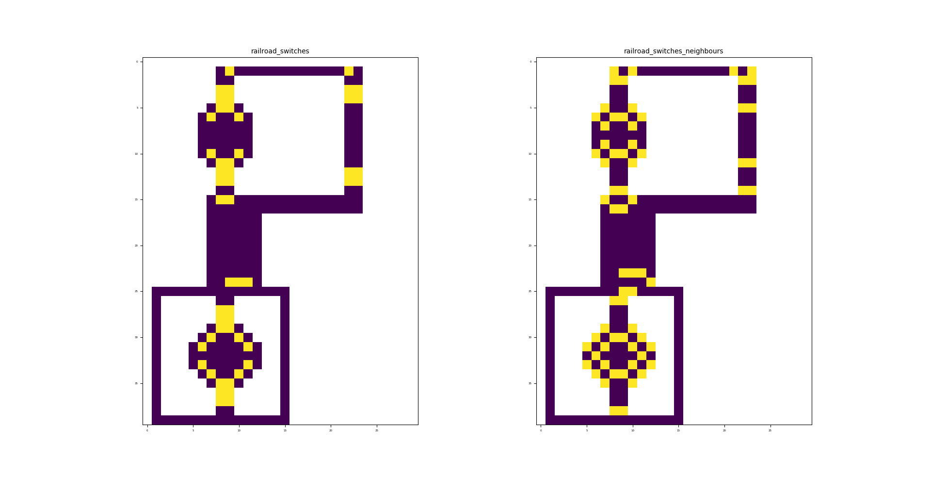
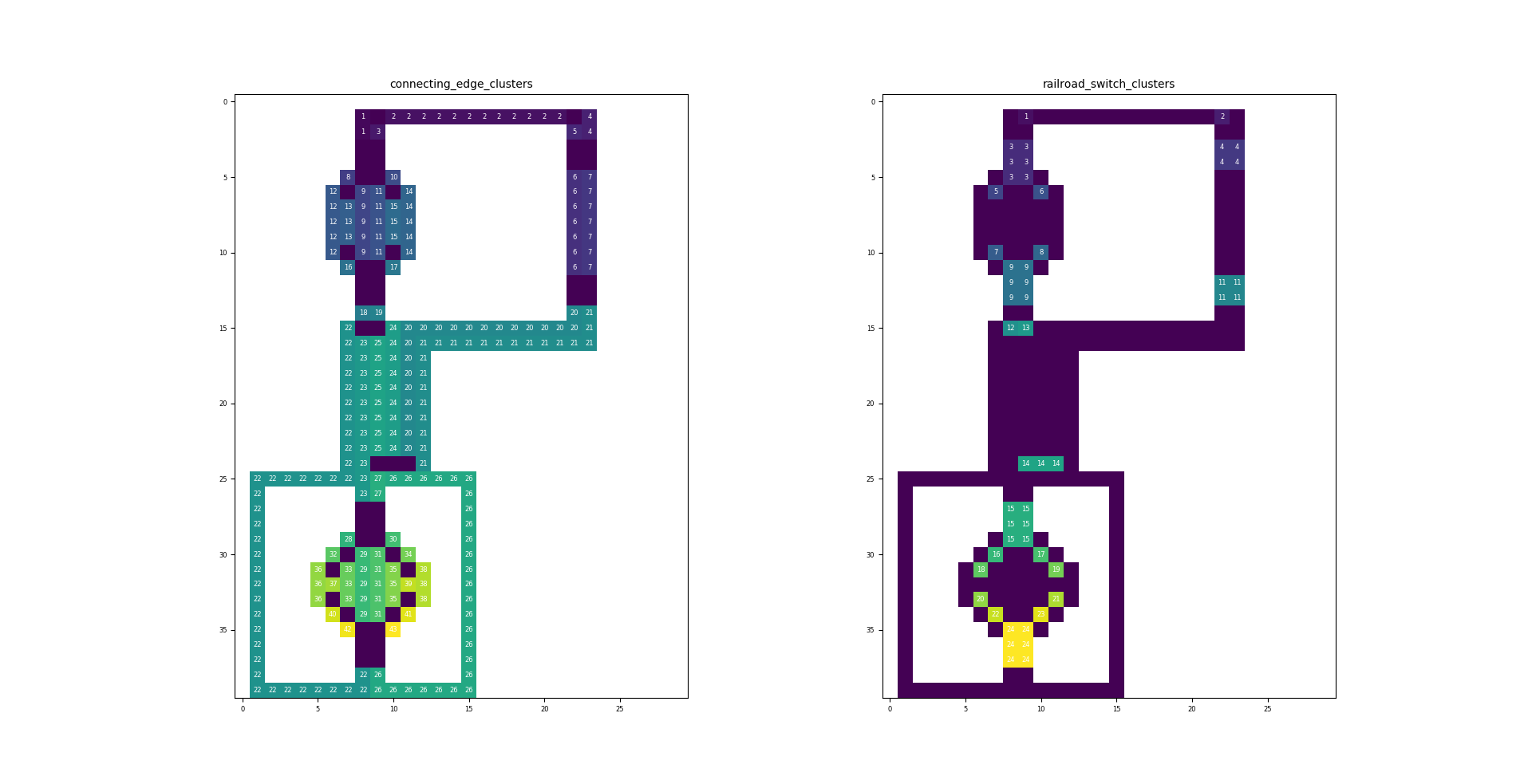
  The illustration on the left shows all crossings (switches) and the illustration on the right shows all switch neighbours. A switch neighbours is an infrastructure element that has an intersection (crossing) as its neighbour.

  

  The figure illustrates the mapping of crossings (switches) and switch neighbours to the infrastructure.

  

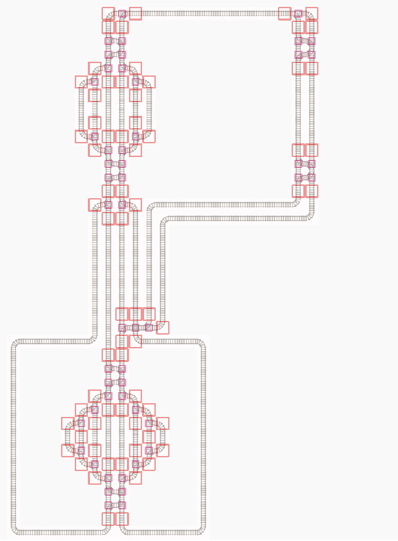
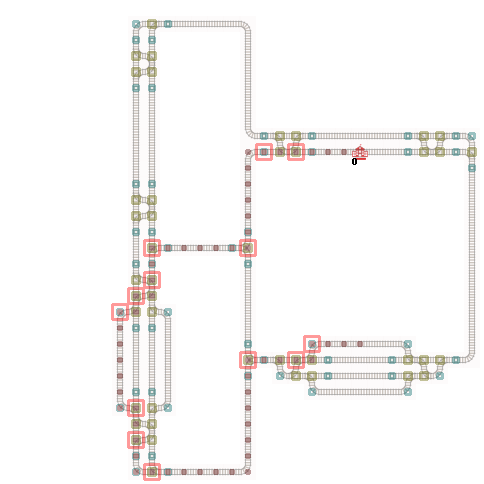
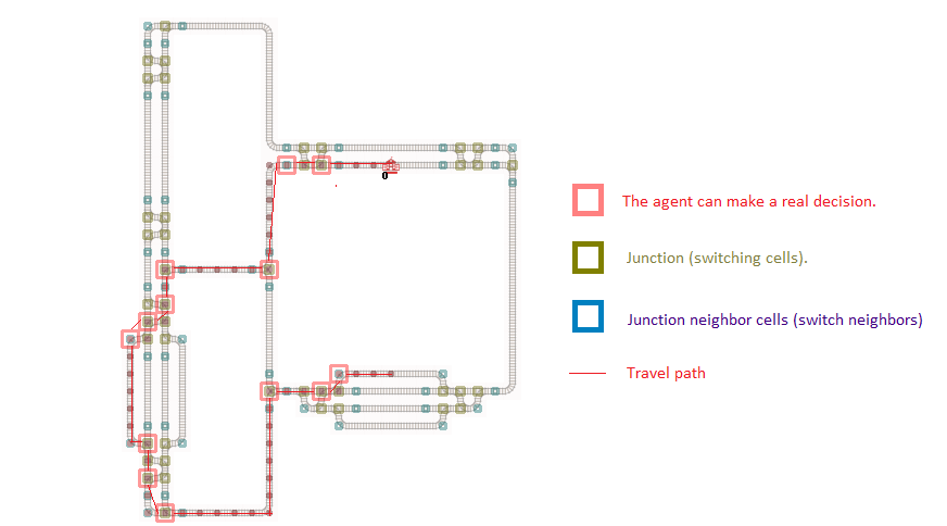
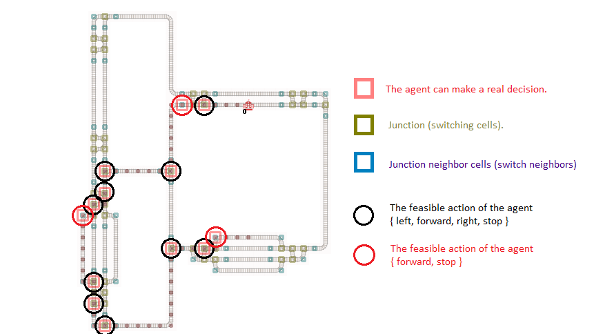
  A detailed example is shown visually below. Which cells are potential decision points, which are real decision points for an agent and which decisions can be made at them. For all other cells it makes sense to choose forward only.

  

  

• RailroadSwitchCluster

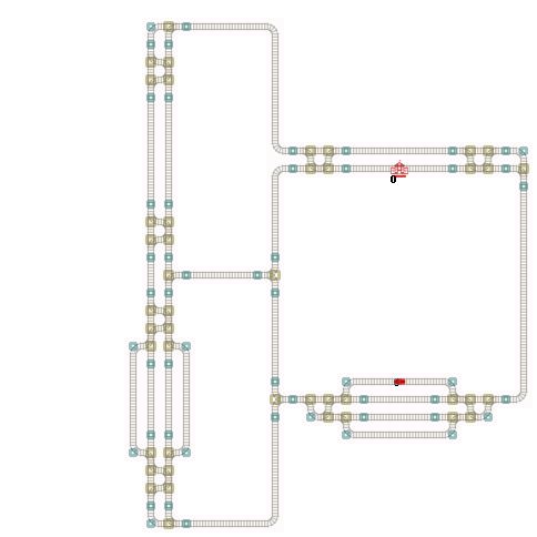
  The left illustration shows all connecting edges (cluster). The number represents the cluster id. Cells with the same cluster id belong to the same cluster. The right illustration shows all switch clusters. A switch cluster contains one or more crossing (switch) cells where each switch within the cluster are all neighbors. The switches in the same cluster have the same switch cluster id.

  

• FlatlandResourceAllocator

  The Flatland Resource Allocator extension allows the implementation of a simultaneous allocation of multiple resources to an agent, and also allows the concept of minimal headway (train-following), which roughly simulates the real infrastructure behavior. A two-minute train sequence (n-flatland time steps) is often used in many real railway systems - the entire system is therefore designed for a minimum headway of n seconds. With the help of the multi-resource allocator it is possible to implement "flank protection", ... and dynamic movement.

• FlatlandGraphBuilder

  

  A Flatland environment can be represented as different kinds of graphs. For example, every cell can be modelled, but also graphs that only include decision cells are useful. For most applications, not only the rail layout but also the available direction options an agent has at a vertex, dependent on its incoming direction (edge), have to be modelled. In that case, a cell is translated into multiple vertices, one for each direction available.

  The FlatlandGraphBuilder converts Flatland's grid cell-based topology into a directed graph g. The graph consists of nodes and edges. An edge is defined by "from-node" u and "to-node" v such that for the edge e = (u, v). A node in the graph is defined by position and direction. The position corresponds to the position of the underlying cell in the original flatland topology, and the direction corresponds to the direction in which an agent reaches the cell. Thus, the node is defined by (x, y, d), where x is the index of the horizontal cell grid position, y is the index of the vertical cell grid position, and d is the direction of cell entry. Based on the grid cell position and the cell entry direction, the connection to the neighboring cell can be estimated. The estimation is done using the pure flatland navigation technique. In the flatland (2d gird), not every of the eight neighbors cell can be reached from every direction. Therefore, the entry direction information is key. In the graph g only edges exist where a feasible transition from node u to node v exist. An edge has several attributes, such as the length of the edges, the resource which can be mutually exclusive used, the flatland action to be chosen to get from node u to node v. The length of the edge is 1 as long as no infrastructure is used. If an infrastructure is used, the infrastructure defines the edge length, which is the by the infrastructure defined length of the flatland cell that lies under node u. The resource is defined as the flatland cell that lies under the node u. The flatland action is the action that must be selected so that an agent at node u (i.e. position and direction) can get to node v.

  With the help of the graph it is very easy to calculate the shortest connection from node A to node B. The API makes it possible to solve such tasks very efficiently. Moreover, the graph can be simplified so that only decision-relevant nodes remain in the graph and all other nodes are merged. A decision node is a node or flatland cell (track) that reasonably allows the agent to stop, go, or branch off. For straight track edges within a route, it makes little sense to wait in many situations. This is because the agent would block many resources, i.e., if an agent does not drive to the decision point: a cell before a crossing, the agent blocks the area in between. This makes little sense from an optimization point of view.

  The implementation uses networkX, so there are also many graph functions available.

• FlatlandDynamics

  The diagram on the left illustrates the speed diagram for each train. The traveled distance [m] is plotted on the x-axis. The speed in kilometers per hour [km/h] is shown on the y-axis. The orange curve shows the maximum allowed speed. The blue curve is the simulated speed. The length of the train is easy to see because the last axle of the train must have allowed a higher speed, otherwise the train will not accelerate. The diagram on the right illustrates the acculeration [m/s] on the y-axis. On the x-axis traveled distance [m] is plotted again. The red colored part of the velocity and acceleration curve shows where the agent has to brake hard due to an active malfunction.

  

• Rolling Stock

  The rolling stock data stores the technical characteristics of each locomotive, including tractive effort and speed limits. The DynamicAgent stores the physical properties such as mass and length of the complete train (agent) and requires the rolling stock data to simulate the tractive effort and acceleration.

  The figure illustrates the traction characteristics. The speed is plotted on the x-axis. The maximum tractive effort is plotted on the y-axis. Traction power is limited by the maximum force that traction can exert on the wheel and is further limited by the maximum power of the motor.

  

  $$F = m a := Force : [kN]$$

  $$P = F v := Power : [kW]$$

  $$v := Velocity : [{ m \over s}]$$

  $$m := Mass : [10^3kg]$$

  $$a := Acceleration : [{m \over s^{2}}]$$

  Where $P_{max}$ is the maximum power of the traction. $P_{max}$ depends on two factors $F_{max}$ and $v_{F_{max}}$. Where $F_{max}$ is the overall maximum force the traction can deliver and where $v_{F_{max}}$ is the speed up to which the vehicle can deliver the maximum force.

  The power consumption (for acceleration) must be positive and less than the maximum power of the traction $P_{max}$ and it cannot exceed the maximum force $F_{max}$.

  $$0 <= P <= P_{max}$$

  $$P_{max} = F_{max} v_{F_{max}}$$

  $$F <= \min({ P_{max} \over v} , F_{max})$$

• FlatlandDynamicsRendering

  Resources colored orange, red or black are occupied by the train. Orange indicates a resource reserved for the train but not required by either the braking distance or the physical train. Red and black resources are security related. Black is the physical train and red resources are needed for braking. The physical train can occupy more than one cell since the train length can be greater than the length of the underlaying cell. In the visualization, however, a train that would fit into one cell can also take up more than one cell if part of the train is in the next cell and part is still in the current one. Green resources are still occupied. They are intended to approximately simulate the time required to handle all security elements - they represents the minimum headway time.

  

  

  The Example is showing a moving block based simulation. The rendering is done with FlatlandDynamicsRenderer.

Working code

• Google coLab notebook - Recife export
• Google coLab notebook - Simulation with multi-resource reservation
• Google coLab notebook - Flatland dynamics

Installation

The code is tested with Python 3.8 - expected to work with higher versions of Python.

Prerequisites (optional)

Install Anaconda and create a new conda environment:

conda create python=3.8 --name flatland-ext
conda activate flatland-ext
pip install flatland-rl

From sources

The Flatland code source is available from AIcrowd gitlab and Flatland railway extension can be found at github:

git clone https://github.com/flatland-association/flatland-rl.git
cd flatland
pip install -r requirements_dev.txt
python setup.py install
cd .. 

git clone https://github.com/aiAdrian/flatland_railway_extension.git/
cd flatland_railway_extension
python setup.py install
cd .. 

Stable release

Install flatland railway extension:

pip install flatland-railway-extension

Test installation

Test that the installation works:

python -c "import flatland_railway_extension.examples.demo_flatland_dynamics"

_{Troubleshooting¹}

Examples

Some examples can be found at: flatland_railway_extension.examples.*

PePy - PyPI Download Stats

Links

Flatland Challenge

Flatland introduction

Rolling stock

Nagel-Schrekenberg-Model

Information

The initial implementation is authored by Adrian Egli's ( aiAdrian) neurips2020 flatland challenge solution (submission)

Permission to use

If you use this or any idea out of this code for/in any academic publication or commercial products - you must credit the authors.

Footnotes

1. On Windows Subsystem for Linux (WSL) you may need to install some additional packages pip install pyvirtualdisplay, pip install piglet and sudo apt install libnvidia-gl-440 to get the rendering working. However, using Flatland Railway Extension with WSL is not recommended, we recommend native Windows or Linux operating system. OS/X is not very well tested yet. ↩