SparseIR.jl - intermediate representation of propagators

This library provides routines for constructing and working with the intermediate representation of correlation functions. It provides:

• on-the-fly computation of basis functions for arbitrary cutoff Λ
• basis functions and singular values accurate to full precision
• routines for sparse sampling

Note Refer also to the accompanying paper:
sparse-ir: Optimal compression and sparse sampling of many-body propagators

Installation

SparseIR can be installed with the Julia package manager. Simply run the following from the command line:

julia -e 'import Pkg; Pkg.add("SparseIR")'

We support Julia version 1.6 and above, and recommend Julia 1.8 or above for optimal performance. We depend on a quad-precision library and an SVD library for the accurate computation of the singular value decomposition, a quadrature library for expansion coefficients and a Bessel functions package for the Fourier transformed basis. All of these are automatically installed. (A formal list of dependencies can be found in Project.toml.)

To manually install the current development version, you can use the following:

julia -e 'import Pkg; Pkg.develop(url="https://github.com/SpM-lab/SparseIR.jl")'

Warning This is recommended only for developers - you won't get automatic updates!

Documentation and tutorial

Check out our comprehensive tutorial, where self-contained notebooks for several many-body methods - GF(2), GW, Eliashberg equations, Lichtenstein formula, FLEX, ... - are presented.

Refer to the API documentation for more details on how to work with the Julia library.

There is also a Python library and (currently somewhat restricted) Fortran library available for the IR basis and sparse sampling.

Example usage

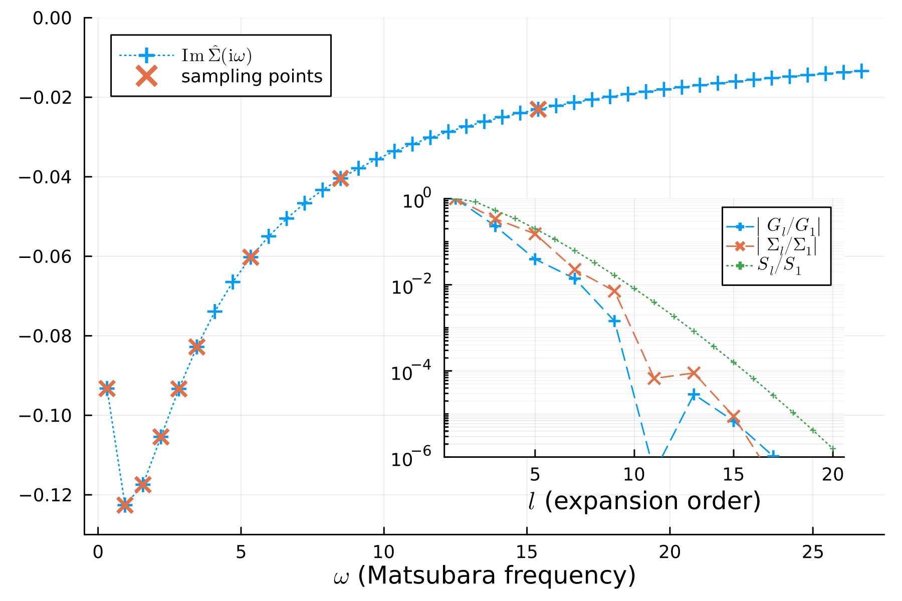
As a simple example, let us perform self-consistent second-order perturbation theory for the single impurity Anderson model at finite temperature. Its Hamiltonian is given by $$H = -\mu(c^\dagger_\uparrow c_\uparrow + c^\dagger_\downarrow c_\downarrow) + U c^\dagger_\uparrow c^\dagger_\downarrow c_\downarrow c_\uparrow + \sum_{p\sigma} \big(V_{p\sigma} f^\dagger_{p\sigma} c_\sigma + V^\star_{p\sigma} c^\dagger_\sigma f_{p\sigma}\big) + \sum_{p\sigma} \epsilon_p f^\dagger_{p\sigma} f_{p\sigma},$$ where $U$ is the electron interaction strength, $\mu$ is the chemical potential, $c_\sigma$ annihilates an electron on the impurity, $f_{p\sigma}$ annihilates an electron in the bath, $\dagger$ denotes the Hermitian conjugate, $p\in\mathbb R$ is bath momentum, and $\sigma\in{\uparrow, \downarrow}$ is spin. The hybridization strength $V_{p\sigma}$ and bath energies $\epsilon_p$ are chosen such that the non-interacting density of states is semi-elliptic with a half-bandwidth of one, $\rho_0(\omega) = \frac2\pi\sqrt{1-\omega^2}$, $U=1.2$, $\beta=10$, and the system is half-filled, $\mu = U/2$.

using SparseIR

function main(β = 10, ωmax = 8, ε = 1e-6)
    # Construct the IR basis and sparse sampling for fermionic propagators
    basis = FiniteTempBasis{Fermionic}(β, ωmax, ε)
    sτ = TauSampling(basis)
    siω = MatsubaraSampling(basis; positive_only=true)
    
    # Solve the single impurity Anderson model coupled to a bath with a
    # semicircular density of states with unit half bandwidth.
    U = 1.2
    ρ₀(ω) = 2/π * √(1 - clamp(ω, -1, +1)^2)
    
    # Compute the IR basis coefficients for the non-interacting propagator
    ρ₀l = overlap.(basis.v, ρ₀)
    G₀l = -basis.s .* ρ₀l
    
    # Self-consistency loop: alternate between second-order expression for the
    # self-energy and the Dyson equation until convergence.
    Gl = copy(G₀l)
    Gl_prev = zero(Gl)
    G₀iω = evaluate(siω, G₀l)
    while !isapprox(Gl, Gl_prev, atol=ε)
        Gl_prev = copy(Gl)
        Gτ = evaluate(sτ, Gl)
        Στ = @. U^2 * Gτ^3
        Σl = fit(sτ, Στ)
        Σiω = evaluate(siω, Σl)
        Giω = @. (G₀iω^-1 - Σiω)^-1
        Gl = fit(siω, Giω)
    end
end

You may want to start with reading up on the intermediate representation. It is tied to the analytic continuation of bosonic/fermionic spectral functions from (real) frequencies to imaginary time, a transformation mediated by a kernel $K$. The kernel depends on a cutoff, which you should choose to be $\Lambda \geq \beta \omega_{\mathrm{max}}$, where $\beta$ is the inverse temperature and $\omega_{\mathrm{max}}$ is the bandwidth.

One can now perform a singular value expansion of this kernel, which generates two sets of orthonormal basis functions, one set $v_\ell(\omega)$ for real frequency side $\omega$, and one set $u_\ell(\tau)$ for the same object in imaginary (Euclidean) time $\tau$, together with a "coupling" strength $s_\ell$ between the two sides.

By this construction, the imaginary time basis can be shown to be optimal in terms of compactness.

License and citation

This software is released under the MIT License. See LICENSE for details.

If you find the intermediate representation, sparse sampling, or this software useful in your research, please consider citing the following papers:

• Hiroshi Shinaoka et al., Phys. Rev. B 96, 035147 (2017)
• Jia Li et al., Phys. Rev. B 101, 035144 (2020)
• Markus Wallerberger et al., SoftwareX 21, 101266 (2023)

If you are discussing sparse sampling in your research specifically, please also consider citing an independently discovered, closely related approach, the MINIMAX isometry method (Merzuk Kaltak and Georg Kresse, Phys. Rev. B 101, 205145, 2020).