strange Ey field using Laser module

[phyax]

Hello,

I am trying to launch a right-hand polarized whistler wave with the laser module. The background plasma is uniform, isotropic and magnetized. The laser module is set to launch a right-hand polarized wave at 0.2 omce (electron gyrofrequency) propagating in +x direction. For the results, I got By, Bz and Ez correctly peaked at 0.2 omce. But Ey has a significant amount of other frequencies. In the plot below, the spectrum of By, Bz, Ez and Ey are shown. Note that the frequency range of Ey is 10 times larger than other components to bring Ey's all significant frequencies. Different colors represent different distance from the antenna.

I checked the polarization of By and Bz. It is right-hand polarized. Please see the hodogram and the field pattern below. Ez shows similar field pattern. But Ey has a substantial amount of smaller wave length components (I did not plot it here).

Here is the python input file for this run. Do you have any idea why such strange Ey field occurs? Thanks.

tst2d_0_antenna.txt

[mccoys]

Hi,

Just an idea that could be tested: could it be caused by the absorbing EM conditions in direction y?

[MickaelGrechX]

Hi! I've just discussed with Fred, and we think we have a possible explanation for your pb. First, as Fred pointed out, you're deal with a plane wave, so we strongly suggest that you use periodic boundary conditions in the y-direction. This will prevent some weird reflection/absorption at the y-boundary that somehow could add some high frequencies in your spectrum as you have a rough cut at the edge. Second, I would not use a constant time profile for your laser field. As you are using a circularly polarized wave this means that you have a sharp cut-off in your one of your electric field (Ey I would guess) and therefore plenty of high frequencies! Rather use something that starts at 0 and increases, e.g. over 1 cycle, up to your constant value a0. I hope this will help! Cheers, Micka

…

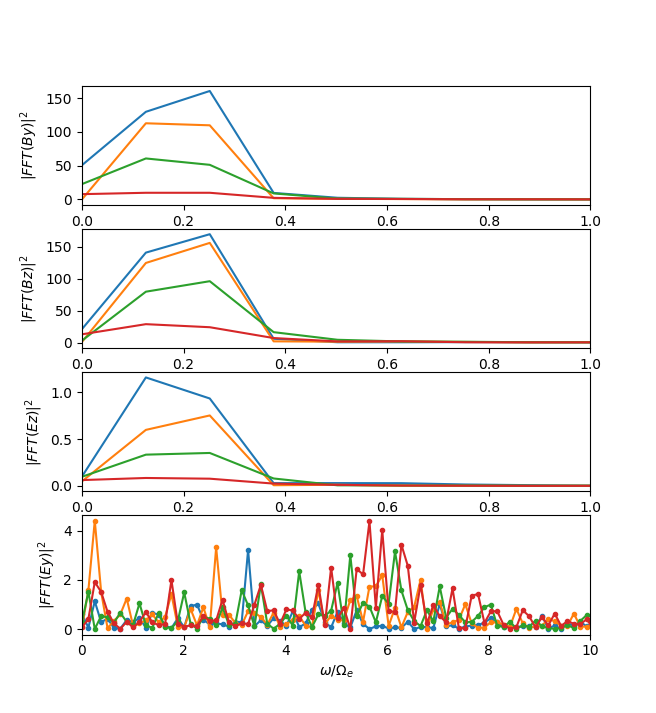
On Fri, Jun 16, 2017 at 12:25 AM, phyax ***@***.***> wrote: Hello, I am trying to launch a right-hand polarized whistler wave with the laser module. The background plasma is uniform, isotropic and magnetized. The laser module is set to launch a right-hand polarized wave at 0.2 omce (electron gyrofrequency) propagating in +x direction. For the results, I got By, Bz and Ez correctly peaked at 0.2 omce. But Ey has a significant amount of other frequencies. In the plot below, the spectrum of By, Bz, Ez and Ey are shown. Note that the frequency range of Ey is 10 times larger than other components to bring Ey's all significant frequencies. Different colors represent different distance from the antenna. [image: spectrum_eb] <https://user-images.githubusercontent.com/20483877/27204001-6c8b421c-51dd-11e7-8925-f2a1274964b1.png> I checked the polarization of By and Bz. It is right-hand polarized. Please see the hodogram and the field pattern below. Ez shows similar field pattern. But Ey has a substantial amount of smaller wave length components (I did not plot it here). [image: hodogram_bybz] <https://user-images.githubusercontent.com/20483877/27204042-a52764f2-51dd-11e7-9a37-b480bbd6c228.png> [image: field_bybz] <https://user-images.githubusercontent.com/20483877/27204048-ab5a7d5a-51dd-11e7-9f5e-4f8083746924.png> Here is the python input file for this run. Do you have any idea why such strange Ey field occurs? Thanks. tst2d_0_antenna.txt <https://github.com/SmileiPIC/Smilei/files/1079149/tst2d_0_antenna.txt> — You are receiving this because you are subscribed to this thread. Reply to this email directly, view it on GitHub <#9>, or mute the thread <https://github.com/notifications/unsubscribe-auth/ARsfTMRfhITHNANhUstDpKrU_oYoUt4Mks5sEa9GgaJpZM4N70IM> .

-- ------------------------------------------------------------- Mickael Grech Chargé de recherche CNRS --- Laboratoire d'Utilisation des Lasers Intenses Ecole Polytechnique Route de Saclay 91128 Palaiseau Cedex, France --- tel.: +33 (0)1 69 33 54 16 gsm: +33 (0)6 95 56 48 43 [email protected] -------------------------------------------------------------

[phyax]

Hi Mickael, Fred,

Thanks for you response.

I tested two cases: (1) same as the case in the first post but change EM boundary condition in y direction to "periodic"; (2) change EM boundary condition in y to "periodic" and use the trapezoidal profile as time profile with slope1= 1 wave cycle and the plateau spanning the remaining time after slope1.

In case (1), the spectrum of Ey looks similar to that in the first post. So these high frequency component in Ey are probably not due to the absorbing boundary condition in y.

in case (2), still, the spectrum of Ey has a substantial amount of high frequency components, similar to that in the first posts. In fact, I think if the high frequency components of Ey are caused by the sharp cut-off in amplitude, then Ez, By and Bz should have these high frequency components too.

I am still not sure why Ey has so many high frequency components. Let me know how you think.

Best,
Xin

[mccoys]

What is the amplitude of Ey compared to the others?

Do you have plots of Ey similar to those you posted for By and Bz?

[phyax]

The amplitude of Ey is about 10 times larger than that of Ez. This could be seen in the spectrum of Ey and Ez in the first post.

Here is the field pattern of Ey and Ez.

[mccoys]

Maybe some 2-stream instability from the particles that you put in the box ?

What happens if you have no particles ? Do you still see the high frequencies ?

[phyax]

Hi all,

Sorry for my silence for some time.

I did a test without particles in the box. The wave propagates as light wave as expected. Ey is correct and I did not see any high frequencies in it.

In my simulation setup, there are only background thermal electrons (Debye length = grid size) and immobile protons. There should be no 2-stream instability. Therefore the strange Ey field here should be caused by the procedure of charge and current deposit.

I only find some benchmark tests for the propagation of a EM wave in vacuum (tst1d_0_em_propagation.py, tst2d_0_em_propagation.py, tst3d_0_em_propagation.py). But there is no benchmark test for the propagation of a EM wave in a magnetized plasma. Could the team test this case as a benchmark? Thanks for your help.

Best regards,
Xin

[phyax]

Attached is my python script for input.

tst2d_em_propagation_plasma.txt

[beck-llr]

Could this be an effect of the 2D geometry ? You are looking at the background noise which is much higher in the X and Y direction (plane of the simulation) than in the Z direction for the electric field (no space charge can build up along Z) and inversely for the magnetic field.

[phyax]

Thanks! I will test a 3D case soon.

[phyax]

Hello,

I tested a 1D and 3D case. In 1D, both Ey and Ez behave as expected. In 2D, Ez behaves as expected but Ey has a lot of large amplitude high frequency components. In 3D, both Ey and Ez has a lot of large amplitude high frequency components and behave "strange". Therefore, I agree with you that it is an effect of dimensions. The "strange" Ey in 2D is due to the space charge built up in y direction (Ez is correct in 2D since no space charge is built up in z direction). Both Ey and Ez are "strange" in 3D because space charge can be built up in both y and z directions.

Unfortunately, since my problem eventually requires nonuniform magnetic field configuration, 1D model cannot do this. But thanks for your help.

Another unrelated question, when the particle boundary condition is specified as "none" and the field boundary condition is "silver-muller", are the particles removed from the memory at the boundary?

[jderouillat]

Concerning the point on particles boundary conditions : I confirm that if silver-muller is selected for fields then the none will apply a supp conditions on particles.

[MickaelGrechX]

Dear Xin, These latest exchanges confirm that your problem comes from the noise inherent to PIC codes. I think that the main problem in your set-up is that the field you initialised has such a small strength (a0<<1). If you want to stick with the PIC approach for this kind of simulation, I would suggest you to (1) use the 4th order for interpolation/projection, (2) strongly increase the number of particle-per-cells (beyond 1000), and (3) potentially try some current smoothing techniques. Otherwise, you could try for Vlasov codes which do not suffer from this noise problem. However, I do not know any open-source code available and that performs nicely in 2D.

…

On Sat, Sep 16, 2017 at 1:51 AM, phyax ***@***.***> wrote: Hello, I tested a 1D and 3D case. In 1D, both Ey and Ez behave as expected. In 2D, Ez behaves as expected but Ey has a lot of large amplitude high frequency components. In 2D, both Ey and Ez has a lot of large amplitude high frequency components. I agree with you: the strange Ey in 2D is due to the space charge built up in x and y direction (Ez is correct in 2D since no space charge is built up in z direction). Unfortunately, since my problem eventually requires nonuniform magnetic field configuration, 1D model cannot do this. But thanks for your help. Another unrelated question, when the particle boundary condition is specified as "none" and the field boundary condition is "silver-muller", are the particles removed from the memory at the boundary? — You are receiving this because you commented. Reply to this email directly, view it on GitHub <#9 (comment)>, or mute the thread <https://github.com/notifications/unsubscribe-auth/ARsfTH8BDjwW6wz1ZohQWb0GVFTlChZEks5siw1kgaJpZM4N70IM> .

-- ------------------------------------------------------------- Mickael Grech Chargé de recherche CNRS --- Laboratoire d'Utilisation des Lasers Intenses Ecole Polytechnique Route de Saclay 91128 Palaiseau Cedex, France --- tel.: +33 (0)1 69 33 54 16 gsm: +33 (0)6 95 56 48 43 [email protected] -------------------------------------------------------------

[phyax]

Thank you all for the responses. Since 4th order for field solver and current smoothing are not available yet in current release of Smilei, I only tried to increase the number of super-particles per cell to reduce the noise. With 400 particles per cell (512 x 512 grids), Ey is 10 times bigger than Ez. With 22500 particles per cell (simulation box is reduce in the transverse direction to finish it in one hour on 8 nodes (36 cores on each nodes), 512 x 16 grids), Ey is 3 times bigger than Ez. Note that Ey is expected to be approximately equal to Ez. I will probably use other approach to tackle my problem. Thanks for your help.

[MickaelGrechX]

4th order projection is actually available in the current release of Smilei (since v3.2 I would say). A current filtering method is also available but has not been yet documented. It corresponds to a N-pass binomial filter in space, and to use it, you just have to add "currentFilter_int=2" (if you want 2 passes). Now, I do not know exactly what it is you want to simulate, but it is not necessarily because you have noise that you cannot use the simulation results. Often, if you look at e.g. parametric instabilities or characteristic waves, you can still clearly see their signatures by diagnosing their growth rate (for inst.) and/or spectra (in \omega, k for instance). Finally, if noise is really a pb for your study, I would turn to Vlasov codes. But, as I said earlier, they may be more difficult to find & most likely more computer resources demanding.

…

On Tue, Sep 19, 2017 at 6:42 AM, phyax ***@***.***> wrote: Thank you all for the responses. Since 4th order for field solver and current smoothing is not available yet in current release of Smilei, I only tried to increase the number of super-particles per cell to reduce the particle. With 400 particles per cell (512 x 512 grids), Ey is 10 times bigger than Ez. With 22500 particles per cell (simulation box is reduce in the transverse direction to finish it in one hour, 512 x 16 grids), Ey is 3 times bigger than Ez. Note that Ey is expected to be approximately equal to Ez. I will probably use other approach to tackle my problem. Thanks for your help. — You are receiving this because you commented. Reply to this email directly, view it on GitHub <#9 (comment)>, or mute the thread <https://github.com/notifications/unsubscribe-auth/ARsfTA2KAbgqFOED4FuYWKqkO4PsNqM1ks5sj0ZKgaJpZM4N70IM> .

-- ------------------------------------------------------------- Mickael Grech Chargé de recherche CNRS --- Laboratoire d'Utilisation des Lasers Intenses Ecole Polytechnique Route de Saclay 91128 Palaiseau Cedex, France --- tel.: +33 (0)1 69 33 54 16 gsm: +33 (0)6 95 56 48 43 [email protected] -------------------------------------------------------------

[phyax]

Thanks Micka. I upgraded to v3.2 and start to use the 4th order interpolation and current filtering. They help mitigate the noise problem. I also noticed that there is an electric field filter mentioned in the Smilei paper on arxiv submitted to CPC. Does this help mitigate the noise and is it available to use in v3.2?

The noise problem matters in my simulation, since my simulation looks at the phase space dynamics of resonant electrons (which will give rise to some triggered emissions) and the amplitude and phase of the electric field matters in this situation.