-
Notifications
You must be signed in to change notification settings - Fork 7
BadD
The standard EPA workflow has problems with data where the likelihood
is weakly identified for the model. Unfortunately, this issue occurs with most
dose-response data. The reason: we usually have 3 dose groups plus the
background dose, and we fit dose-response models with
library(knitr)

doses<- c(0,0,0,0,0.156,0.156,0.156,0.3125,0.3125,0.3125,
          0.625,0.625,0.625,1.25,1.25,1.25,2.5,2.5,2.5,5,5,
          5,5,10,10,10,10,20,20,20,20)

resp <- c(3.972915,3.866893,3.772929,3.417624,3.473904,3.978128,3.917840,
          3.976679,3.721169,3.637042,4.097541,3.602818,3.544474,3.680584,
          3.335199,3.986959,2.526221,2.837538,3.643890,3.345252,3.543438,
          2.957502,2.916890,3.665053,2.334471,2.962853,3.015622,2.840253,
          2.707142,2.711778,3.084766)

means <- aggregate(x=resp,by=list(doses),FUN=mean)
sds   <- aggregate(x=resp,by=list(doses),FUN=sd)
library(ggplot2)
M2           <- matrix(0,nrow=nrow(sds),ncol=4)
colnames(M2) <- c("Dose","Resp","N","StDev")
library(ToxicR)
M2[,1] <- means$Group.1
M2[,2] <- means$x
M2[,3] <- as.numeric(table(doses))
M2[,4] <- sds$x
The following data comes from toxicogenomic PFOA exposure data from Gwinn et al. (2020), where we investigate the GLIPR1 receptor's response. This study is unique in that we have 8 non-control dose groups, which is rare. Note: in this case, the model is still ill-defined, and this behavior happens all of the time in toxicogenomic data when you have 3000+ dose-responses to fit. Let's look at the fits; where we note that all models fit the data acceptably.
model1 = single_continuous_fit(M2[,1,drop=FALSE], M2[,2:4], BMR_TYPE="sd", BMR=1,
                              distribution = "normal",fit_type="mle",model_type = "exp-5",degree=2)
AIC_exp5 = -model1$maximum + 2*summary(model1)$GOF[1,2]

model2 = single_continuous_fit(M2[,1,drop=FALSE], M2[,2:4], BMR_TYPE="sd", BMR=1,
                              distribution = "normal",fit_type="mle",model_type =                                    "hill",degree=2)
AIC_hill = -model2$maximum + 2*summary(model2)$GOF[1,2]

model3 = single_continuous_fit(M2[,1,drop=FALSE], M2[,2:4], BMR_TYPE="sd", BMR=1,
                              distribution = "normal",fit_type="mle",model_type = "polynomial",degree=1)
## WARNING: Polynomial models may provide unstable estimates because of possible non-monotone behavior.
AIC_lin = -model3$maximum + 2*summary(model3)$GOF[1,2]
G = matrix( c(model1$bmd,model2$bmd,model3$bmd),byrow=TRUE,ncol=3)
colnames(G) <- c("BMD","BMDL","BMDU")
b <- data.frame(Model=c("Exponential 5","Hill","Linear") ,AIC=c(AIC_exp5,AIC_hill,AIC_lin),
                BMD = G[,1],BMDL=G[,2],BMDU=G[,3])

kable(b,digits=3)| Model | AIC | BMD | BMDL | BMDU |
|---|---|---|---|---|
| Exponential 5 | 2.391 | 1.583 | 0.871 | 2.439 |
| Hill | 2.390 | 1.359 | 1.148 | 2.395 |
| Linear | 1.102 | 7.681 | 5.472 | 12.798 |
We would pick the AIC with the EPA's default approach, but this is problematic. The data have an asymptote; a linear model is not biologically reasonable because it does not pick up this asymptote. Look at the following three plots fit using maximum likelihood estimation. The two models that allow for an asymptote (Hill and Exponential-5) have a much lower BMD (1.38 (0.87) and 1.58 (1.15)) as compared to the Linear model (7.68 (5.47)).
plot(model1)
plot(model2)
plot(model3)
The issue comes from the fact that the linear model is too simple,
but it describes the data well 'enough' given the variability. Further
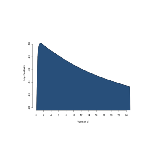
issues come from the fact that there is no information on the 'shape' parameter.
For the Hill model,

After
The problem disappears after adding a little Bayesian information. In fact,
if I add a diffuse caucy prior over the shape parameter, we get a unique maximum.
Now we get a best estimate of about

prior <- create_prior_list(normprior(0,1,-100,100),
                           normprior(0,1,-1e4,1e4),
                           lnormprior(0,1, 0, 100),
                           cauchyprior(0,1,0,18),
                           normprior(0, 10,-100,100));

p_hill_norm = create_continuous_prior(prior,"hill","normal")

cauchy_hill = single_continuous_fit(M2[,1,drop=FALSE], M2[,2:4], BMR_TYPE="sd", BMR=1,
                              distribution = "normal",fit_type="laplace",prior=p_hill_norm)

plot(cauchy_hill)
A Bayesian solution doesn't necessarily obviate the model selection problem. What do you do when multiple models are 'equal?' In the above, the AIC only differed by about 1. The best solution when using parametric models is to use model averaging. With ToxicR this is relatively simply done
MA_ORIG = ma_continuous_fit(M2[,1,drop=FALSE], M2[,2:4], BMR_TYPE="sd", BMR=1,fit_type="mcmc",
                            EFSA=FALSE)
## NOTE: Parameter 'c' added to prior list. It is not used in the analysis.
## NOTE: Parameter 'c' added to prior list. It is not used in the analysis.
## NOTE: Parameter 'c' added to prior list. It is not used in the analysis.
summary(MA_ORIG)## Summary of single MA BMD
##
## Individual Model BMDS
## Model BMD (BMDL, BMDU) Pr(M|Data)
## ___________________________________________________________________________________________
## Hill Distribution: Normal 2.10 (0.75 ,6.46) 0.365
## Exponential-3 Distribution: Normal 4.95 (1.39 ,12.99) 0.312
## Exponential-5 Distribution: Normal 4.67 (1.37 ,13.19) 0.152
## Power Distribution: Normal 7.50 (2.16 ,16.60) 0.077
## Exponential-5 Distribution: Log-Normal 7.14 (2.30 ,18.30) 0.050
## Exponential-3 Distribution: Log-Normal 8.58 (2.58 ,19.00) 0.043
## Hill Distribution: Normal-NCV 3.66 (0.93 ,347.11) 0.000
## Exponential-3 Distribution: Normal-NCV 11.95 (4.06 ,33.26) 0.000
## Exponential-5 Distribution: Normal-NCV 10.70 (3.31 ,47.56) 0.000
## Power Distribution: Normal-NCV 13.82 (5.63 ,32.69) 0.000
## ___________________________________________________________________________________________
## Model Average BMD: 3.93 (1.00, 13.29) 90.0% CI
MA_EFSA = ma_continuous_fit(M2[,1,drop=FALSE], M2[,2:4], BMR_TYPE="sd", BMR=2,EFSA=TRUE,
                            fit_type = "mcmc")
summary(MA_EFSA)
## Summary of single MA BMD
##
## Individual Model BMDS
## Model BMD (BMDL, BMDU) Pr(M|Data)
## ___________________________________________________________________________________________
## Gamma-EFSA Distribution: Normal 9.26 (3.60 ,37.49) 0.241
## LMS Distribution: Normal 5.40 (1.82 ,148.66) 0.212
## Hill-Aerts Distribution: Normal 5.28 (1.84 ,1294.09) 0.193
## Exponential-Aerts Distribution: Normal 9.88 (2.41 ,278.09) 0.079
## Inverse Exponential-Aerts Distribution: Normal 4.07 (1.87 ,2741.33) 0.074
## Lognormal-Aerts Distribution: Normal 4.06 (1.75 ,33.77) 0.072
## LMS Distribution: Log-Normal 17.41 (3.48 ,322.34) 0.029
## Hill-Aerts Distribution: Log-Normal 16.61 (2.92 ,73230.75) 0.023
## Logistic-Aerts Distribution: Normal 14.03 (6.86 ,28.12) 0.020
## Gamma-EFSA Distribution: Log-Normal 14.30 (4.87 ,148.12) 0.012
## Exponential-Aerts Distribution: Log-Normal 18.01 (3.99 ,80.38) 0.011
## Probit-Aerts Distribution: Normal 14.42 (7.46 ,27.47) 0.011
## Inverse Exponential-Aerts Distribution: Log-Normal 28.04 (3.47 ,32353.36) 0.009
## Lognormal-Aerts Distribution: Log-Normal 22.27 (3.32 ,521.71) 0.008
## Logistic-Aerts Distribution: Log-Normal 19.92 (8.66 ,38.81) 0.003
## Probit-Aerts Distribution: Log-Normal 21.29 (9.27 ,45.34) 0.002
## ___________________________________________________________________________________________
## Model Average BMD: 7.53 (2.07, 150.21) 90.0% CI
We now use the models proposed by the European Food Safety Authority. Using EFSA=FALSE you can use the origional models.
plot(MA_ORIG)## Scale for x is already present.
## Adding another scale for x, which will replace the existing scale.

plot(MA_EFSA)## Scale for x is already present.
## Adding another scale for x, which will replace the existing scale.
## Warning: Removed 1 rows containing missing values (`geom_text()`).
## Removed 1 rows containing missing values (`geom_text()`).
## Removed 1 rows containing missing values (`geom_text()`).
## Removed 1 rows containing missing values (`geom_text()`).
## Removed 1 rows containing missing values (`geom_text()`).
## Removed 1 rows containing missing values (`geom_text()`).

