Home
Welcome to the Advanced supervised PCA function SupervisedPCA Wiki
PCA problem
PCA generalisation
Property of Laplacian matrix
Advanced supervised PCA
Generalisation of Advanced supervised PCA
Criteria of cluster validity
Caliński and Harabasz index
The Davies - Bouldin index
The Dunn index family
Fuzzy hypervolume
The Xie - Beni index
The Fukuyama - Sugeno index
Cluster separation with Advanced supervised PCA
Artificial set 1
Artificial set 2
Breast cancer data set
Method behaviour investigation
Required number of PCs
References
Let us consider set of points ![]() where each row xi of matrix X is one observation. Let us consider centred points:
where each row xi of matrix X is one observation. Let us consider centred points: ![]()
There are four standard definitions of Principal Components (PC) [1]. Let us consider a linear manifold Mk of dimension k in the parametric form Mk = {v0+b1v1+...+bkvk|bi∈R}, vk∈Rm, and {v1,...,vk} is a set of orthonormal vectors in Rm. Let us denote dot product as (·,·).
It can be easily shown that for centred data we always have v0=0.
Definition of PCA problem #1 (data approximation by lines and planes): PCA problem consists in finding such sequence Mk, k=1,...,p that the sum of squared distances from data points to their orthogonal projections on Mk is minimal over all linear manifolds of dimension k embedded in Rm:

Definition of PCA problem #2 (variance maximisation): For a set of vectors X and for a given vi, let us construct a one-dimensional distribution Bi={b:b=(x,vi ), x∈X}. Then let us define empirical variance of X along vi as var(Bi), where var() is the standard empirical variance. PCA problem consists in finding such Mk that the sum of empirical variances of X along v1,...,vk would be maximal over all linear manifolds of dimension k embedded in Rm:

Let us consider an orthogonal complement {vk+1,...,vm} of the basis {v1,...,vk}. Then an equivalent definition (minimization of residue variance) is

Definition of PCA problem #3 (mean point-to-point squared distance maximisation): PCA problem consists in finding such sequence of Mk that the mean point-to-point squared distance between the orthogonal projections of data points on Mk is maximal over all linear manifolds of dimension k embedded in Rm:

Having in mind that all orthogonal projections onto lower-dimensional space lead to contraction of all point-to-point distances (except for some that do not change), this is equivalent to minimisation of mean squared distance distortion:

Definition of PCA problem #4 (correlation cancellation): Find such an orthonormal basis {v1,...,vk} in which the covariance matrix for x is diagonal. Evidently, in this basis the distributions (vi,x) and (vj,x), for i≠j, have zero correlation.
Equivalence of the above-mentioned definitions in the case of complete data and Euclidean space follows from Pythagorean Theorem and elementary algebra.
In this paper we use the third definition of PCA problem.
Standard PCA is implemented in SupervisedPCA function. To use standard PCA it is necessary to specify 'usual' in the parameter kind. It is necessary to stress that fastest PCA function is svd and SupervisedPCA is essentially slower.
There are many generalisation of PCA [1]. In SupervisedPCA we implement four of them. In this section we consider problem of search of p principal components.
Normalised PCA [3] requires value 'norm' in the parameter kind. This generalisation is one of the possible weighted PCA with weights equal one divide by distance between points:

This version of PCA is more robust and similar to PCA in l1 norm.
Supervised PCA [3] is defined for classification problem. Let us consider case when each point belongs to one of k classes L1,...,Lk. Let us change requirement of maximal sum of squared distances of projection of data points onto linear manifold by consideration of pairs with points in different classes only:

To use supervised PCA it is necessary to specify value 'super' in parameter kind of SupervisedPCA.
Supervised normalised PCA combines both ideas of supervised and normalised PCA:

The most sophisticated method is Advanced supervised PCA (ASPCA) which is described below. To use ASPCA it is necessary to specify value of α in parameter kind.
We want to find linear manifold in which distances between points of different classes are big and distances between points of the same class are small.
This problem is considered in [1] and [2]. In formulas derivation we follows approach of [3].
Let us consider target functional in form

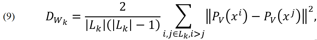
where DB is mean squared distance between points of different classes and DWi is mean squared distance between points of class i:
and
and α is parameter which define relative cost of closeness of points of the same class in comparison to distance of points of different classes. Properties of ASPCA are described in section �Required number of PCs�. All formulas are derived below. It is necessary to stress that usual PCA is not partial case of ASAP but supervised PCA corresponds to ASPCA with α=0.
Let us have Laplacian matrix ![]() :
:

Let us have data matrix ![]() . Each vector xi is row of matrix X.
. Each vector xi is row of matrix X.
For any x=(x1,...,xn) we can calculate

After applying the property (1) we have

Now we can calculate

Let us consider set of points ![]() with two labels (classes). Indices of points with label 1 belongs to set L1 and indices of point with label 2 belongs to set L2. Let us denote the power of set S as |S|. We want to find the low dimensional linear manifold with maximal distances between projections of points of different sets and minimal distances between projection points of the same set.
Let us consider centred data:
with two labels (classes). Indices of points with label 1 belongs to set L1 and indices of point with label 2 belongs to set L2. Let us denote the power of set S as |S|. We want to find the low dimensional linear manifold with maximal distances between projections of points of different sets and minimal distances between projection points of the same set.
Let us consider centred data:

Let us consider set of column vectors ![]() where
where ![]() if
if ![]() and
and ![]() is Kronecker delta. Projection of data points onto p dimensional subspace is
is Kronecker delta. Projection of data points onto p dimensional subspace is
Squared distance between projections of two points xi and xj is
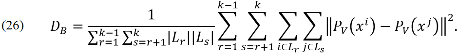
Average squared distance between projections of points of different sets is

Average of squared distances inside one set is
Function of interest can be written as

Alternative way is
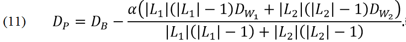
Function (10) takes into account equal contribution of internal distances for two classes and function (11) takes into account equal contribution of all pairs of points of the same class. To simplify algebra we introduce
For function (10) Laplacian matrix has elements:

In accordance with (4):

For optimization function (11) we have formula

for Laplacian matrix with elements

Further we consider problem (10) because for problem (11) results are the same.
Theorem II.1 from [3] states: Let A be an ![]() symmetric matrix. Denote by
symmetric matrix. Denote by
![]() its sorted eigenvalues, and by u1,...,un the corresponding eigenvectors. Then set of vectors u1,...,up is the maximizer of the constrained maximization problem
its sorted eigenvalues, and by u1,...,un the corresponding eigenvectors. Then set of vectors u1,...,up is the maximizer of the constrained maximization problem

subject to:
In accordance with (14), (12) and (6) we can write


Matrices (13) and (16) are symmetrical. It means that matrix
is symmetrical too because property (1):
In accordance with Theorem II.1 from [1] we can conclude that solution of problems (10) and (11) are the set of the p eigenvectors of matrix A with greatest values of eigenvalues. For problem (10) matrix A is
where ![]() is defined by formula (13) and for problem (11) matrix A is
is defined by formula (13) and for problem (11) matrix A is
where ![]() is defined by formula (16).
is defined by formula (16).
In previous section Advanced supervised PCA is defined for problem with two classes. To generalize this method for k classes we need to define: Li is index of points with label i (points of class i). Functions of interest are

where DB is
Laplacian matrices for problems (24) and (25) are defined as

There are several types of cluster validity measures [2]: external, internal and relative. External criteria compare result of clustering algorithm application with a priori knowledge of classes. Internal criteria evaluate quality of clustering structure by data only. Relative criteria compare results of application of two clustering algorithms.
We do not apply any clustering algorithms but simple project data to different linear subspaces. It means that we can consider labels as clustering structure and we cannot apply external criteria. We can apply internal criteria to depict regularity and relative criteria to compare projections onto two different low dimensional linear subspaces.
We will consider predefined classes as clusters in projection. Greater validity of classes means better projection. Let us define several useful values:
Mean of class is

Sum of squared class error is

Class covariance is

Caliński and Harabasz index [5] (greater means better) is defined as:

The Davies - Bouldin index [6] (less means better):

In this study the Dunn index family [7] includes 12 criteria (greater means better):

where D(Li, Lj ) is distance between two classes and can be calculated by one of the following formulas

and diam(Li) is diameter of class and can be calculated as

Fuzzy hypervolume [8] (less means better):

Unfortunately this criterion cannot be used because there is no MatLab implementation of determinant with appropriate accuracy.
The Xie - Beni index [9] (less means better):

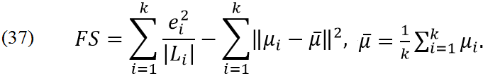
The Fukuyama - Sugeno index [10] (less means better),
In problems (25) and (26) we have one free parameter α. If α=-1 then we have problems which are very similar to standard PCA. For α=0 we have simple supervised PCA [3]. For positive α we have new behaviour.
Let us consider the changes of clusters separability with changing of parameter α. To estimate separability of clusters it is necessary to apply cluster validity measures described in previous section.
We use three dataset to check the work of the method: breast cancer dataset [11] with 30 attributes, 569 cases and 2 classes and two artificial datasets generated by function SupervisedPCATestGeneratorND, presented in the [12] with parameters:
SupervisedPCATestGeneratorND( 10, 2, 100, 20, 1, 0.3, 2)
and
SupervisedPCATestGeneratorND( 10, 3, 100, 20, 1, 0.3, [2, 3]).
Changing of projections onto horizontal line (the first PC) for different α is presented in Figure 1. Figure 2 shows graphs of different measures of cluster validity for one dimensional projection of artificial data set. We can see that all measures of cluster validity are consistent and shows significant changes of validity for 0.6ââ�°Â¤αââ�°Â¤0.67.

Figure 1. Changing of projections onto the first principal component (horizontal axis) for different values of α: a -1, b 0, c 0.61, d 0.63, e 0.65

Figure 2. Cluster validity criteria for different α for one dimensional projection of artificial data set: a Caliński and Harabasz index, b Davies - Bouldin index (blue), Xie - Beni index (red) and Fuzzy hypervolume (yellow), c Fukuyama - Sugeno index and d, e and f Dunn index with different measures of distance between clusters and diameter of cluster.

Figure 3. Cluster validity criteria for different α for two dimensional projection of artificial data set: a Caliński and Harabasz index, b Davies - Bouldin index, c Xie - Beni index, d Fuzzy hypervolume (yellow), e Fukuyama - Sugeno index and f, g and h Dunn index with different measures of distance between clusters and diameter of cluster.
Figure 3 shows graphs of different measures of cluster validity for two dimensional projection of artificial data set. We can see that all measures of cluster validity are consistent and shows significant changes of validity for 0.98ââ�°Â¤αââ�°Â¤1. Figure 4 shows graphs of different measures of cluster validity for tree dimensional projection of artificial data set. We can see that all measures of cluster validity are consistent and shows significant changes of validity for 0.98ââ�°Â¤αââ�°Â¤1.

Figure 4. Cluster validity criteria for different α for three dimensional projection of artificial data set: a Caliński and Harabasz index, b Davies - Bouldin index, c Xie - Beni index, d Fuzzy hypervolume (yellow), e Fukuyama - Sugeno index and f, g and h Dunn index with different measures of distance between clusters and diameter of cluster.
Figure 5 shows changing of cluster validity criteria for artificial dataset for different dimension of projection. We can see that the best result corresponds to one dimensional projection. It is true for the first artificial data set.

Figure 5. Graph of validity criteria for different dimensions for α=10.
Figure 6 shows graphs of different measures of cluster validity for one dimensional projection of artificial data set. We can see that all measures of cluster validity are consistent and shows significant changes of validity. Values of optimal α for each measure are presented in Table 1. Corresponding one dimensional projections are presented in Figure 7.

Figure 6. Cluster validity criteria for different α for one dimensional projection of artificial data set: a Caliński-Harabasz index, b Davies - Bouldin index, c Xie - Beni index, d Fuzzy hypervolume, e Fukuyama - Sugeno index and f-q Dunn index with different measures of distance between clusters and diameter of cluster.
Table 1. Optimal α for different cluster validity criteria for one dimensional projections
| Cluster validity criterion | Fig | α | Cluster validity criterion | Fig | α | |
| Dunn index 8 | m | 0.13 | Davies-Bouldin index | b | 3.33 | |
| Dunn index 5 | j | 0.52 | Caliski-Harabasz index | a | 50 | |
| Fuzzy hypervolume | d | 1 | Fukuyama-Sugeno index | e | 50 | |
| Dunn index 11 | p | 1.32 | Dunn index 1 | f | 50 | |
| Dunn index 4 | i | 1.65 | Dunn index 2 | g | 50 | |
| Dunn index 7 | l | 1.65 | Dunn index 3 | h | 50 | |
| Dunn index 10 | o | 1.65 | Dunn index 6 | k | 50 | |
| Xie-Beni index | c | 2.67 | Dunn index 9 | n | 50 | |
| Dunn index 12 | q | 2.93 |

Figure 7. Changing of projections onto the first principal component (horizontal axis) for different values of α: a 0.13, b 0.52, c 1, d 1.32, e 1.65, f 2.67, g 2.93, h 3.33 and i 50.
Figure 8 shows graphs of different measures of cluster validity for two dimensional projection of artificial data set. We can see that all measures of cluster validity are consistent and shows significant changes of validity. Values of optimal α for each measure are presented in Table 2. Corresponding two dimensional projections are presented in Figure 9.

Figure 8. Cluster validity criteria for different α for two dimensional projection of artificial data set: a Caliński-Harabasz index, b Davies - Bouldin index, c Xie - Beni index, d Fuzzy hypervolume (yellow), e Fukuyama - Sugeno index and f-q Dunn index with different measures of distance between clusters and diameter of cluster.
Table 2. Optimal α for different cluster validity criteria
| Cluster validity criterion | Fig | α | Cluster validity criterion | Fig | α | |
| Dunn index 5 | j | -1 | Xie-Beni index | c | 1.52 | |
| Dunn index 7 | l | -1 | Dunn index 4 | i | 1.68 | |
| Dunn index 8 | m | -1 | Dunn index 6 | k | 22.56 | |
| Dunn index 12 | q | -1 | Calinski-Harabasz index | a | 50 | |
| Dunn index 2 | g | -0.82 | Fukuyama-Sugeno index | e | 50 | |
| Dunn index 11 | p | -0.82 | Dunn index 1 | f | 50 | |
| Fuzzy hypervolume | d | 1 | Dunn index 3 | h | 50 | |
| Dunn index 10 | o | 1.48 | Dunn index 9 | n | 50 | |
| Davies-Bouldin index | b | 1.52 |

Figure 9. Changing of projections onto the first two principal component (horizontal axis corresponds to the first component and vertical axis corresponds to the second component) for different values of α: a -1, b -0.82, c 1, d 1.48, e 1.52, f 1.68, g 22.56 and h 50.
The best result of manual search of separated clusters is presented in Figure 10 and comparison of cluster validity criteria is presented in Table 3. We can see that manual finding contains three isolated clusters but this structure is worse than projections which are presented in Figure 9 for all criteria. Unfortunately we cannot use manual search for high dimensional data.

Figure 10. The best result of manual search of separated clusters in 2D projections
Table 3. Comparison of cluster validity criteria for automatic and manual search
| Criterion | Fig | Automatic | Manual |
| Calinski-Harabasz index | a | 3972.823 | 50.779 |
| Davies-Bouldin index | b | 3.694 | 7.761 |
| Xie-Beni index | c | 0.007 | 0.030 |
| Fuzzy hypervolume | d | -204.869 | -63.241 |
| Fukuyama-Sugeno index | e | 8381.604 | 61751.216 |
| Dunn index 1 | f | 0.297 | 0.089 |
| Dunn index 2 | g | 0.415 | 0.208 |
| Dunn index 3 | h | 10.780 | 1.326 |
| Dunn index 4 | i | 1.080 | 0.307 |
| Dunn index 5 | j | 2.038 | 0.714 |
| Dunn index 6 | k | 21.075 | 4.553 |
| Dunn index 7 | l | 0.509 | 0.254 |
| Dunn index 8 | m | 1.039 | 0.589 |
| Dunn index 9 | n | 15.953 | 3.758 |
| Dunn index 10 | o | 0.281 | 0.108 |
| Dunn index 11 | p | 0.568 | 0.250 |
| Dunn index 12 | q | 3.684 | 1.598 |
Visualisation of Breast cancer dataset is presented in Figure 11 and Figure 12.

Figure 11. Projections of Breast cancer data onto space of the two first advanced principal components for different value of α: a) -1, b) 0 (supervised PCA) c) 1 and d) 5

Figure 12. Breast cancer database: a in space of the two first features, b in the space of the two first usual PC, and c in the space of the two first advanced supervised PCs
Table 4 contains eigenvalues of matrix (22) for two value of α for three data set. We can see that for artificial data sets for α=0.99 most of eigenvalues really equal to zero because value 10-16 belongs to interval of rounding error. Artificial 1 dataset is approximately one dimensional and Artificial 2 dataset is approximately two dimensional. We observe the same number of positive eigenvalues for these datasets when α=1. For α=5/3 all eigenvalues exclude one are negative. Value of α for which all eigenvalues become negative is different for different datasets: 7 for Breast cancer, 171 for Artificial 1 and 109 for Artificial 2.
Table 4. Eigenvalues of matrix (22) for two value of α for three data set
| Data set | Breast cancer | Artificial 1 | Artificial 2 | ||||
| α | 0.99 | 1 | 0.99 | 1 | 0.99 | 1 | 5/3 |
| 1 | 0.999889 | 1.000094 | 1 | 1.029187 | 0.79322 | 0.798897 | 5.161371 |
| 2 | 9.97×10⁻⁵ | -8.44×10⁻⁵ | 2.01×10⁻¹⁸ | -0.028638 | 0.20678 | 0.205582 | -3.726389 |
| 3 | 9.75×10⁻⁶ | -8.27×10⁻⁶ | 2.01×10⁻¹⁸ | -4.14×10⁻⁵ | 5.65×10⁻¹⁸ | -2.60×10⁻⁵ | -0.313090 |
| 4 | 8.87×10⁻⁷ | -7.26×10⁻⁷ | 5.15×10⁻¹⁹ | -9.29×10⁻⁵ | 5.65×10⁻¹⁸ | -2.76×10⁻⁵ | -0.000165 |
| 5 | 4.95×10⁻⁷ | -3.01×10⁻⁷ | -5.61×10⁻¹⁹ | -8.50×10⁻⁵ | 1.64×10⁻¹⁸ | -2.89×10⁻⁵ | -0.024547 |
| 6 | 3.87×10⁻⁸ | -2.77×10⁻⁸ | -2.71×10⁻¹⁸ | -7.95×10⁻⁵ | -5.47×10⁻¹⁸ | -3.21×10⁻⁵ | -0.023068 |
| 7 | 2.29×10⁻⁸ | -1.52×10⁻⁸ | -2.71×10⁻¹⁸ | -5.33×10⁻⁵ | -8.10×10⁻¹⁸ | -3.58×10⁻⁵ | -0.021013 |
| 8 | 4.72×10⁻⁹ | -3.24×10⁻⁹ | -1.63×10⁻¹⁷ | -6.97×10⁻⁵ | -9.28×10⁻¹⁸ | -3.78×10⁻⁵ | -0.016608 |
| 9 | 2.07×10⁻⁹ | -1.61×10⁻⁹ | -1.43×10⁻¹⁶ | -6.49×10⁻⁵ | -9.28×10⁻¹⁸ | -4.20×10⁻⁵ | -0.017492 |
| 10 | 1.03×10⁻⁹ | -6.09×10⁻¹⁰ | -2.26×10⁻¹⁶ | -6.20×10⁻⁵ | -8.76×10⁻¹⁶ | -0.00425 | -0.018999 |
| 11 | 4.32×10⁻¹⁰ | -2.84×10⁻¹⁰ | |||||
| 12 | 9.52×10⁻¹¹ | -6.56×10⁻¹¹ | |||||
| 13 | 4.12×10⁻¹¹ | -3.03×10⁻¹¹ | |||||
| 14 | 2.76×10⁻¹¹ | -1.89×10⁻¹¹ | |||||
| 15 | 1.72×10⁻¹¹ | -1.26×10⁻¹¹ | |||||
| 16 | 8.15×10⁻¹² | -5.40×10⁻¹² | |||||
| 17 | 4.64×10⁻¹² | -2.68×10⁻¹² | |||||
| 18 | 2.91×10⁻¹² | -1.86×10⁻¹² | |||||
| 19 | 2.26×10⁻¹² | -1.30×10⁻¹² | |||||
| 20 | 2.08×10⁻¹² | -1.34×10⁻¹² | |||||
| 21 | 9.82×10⁻¹³ | -6.25×10⁻¹³ | |||||
| 22 | 7.21×10⁻¹³ | -4.57×10⁻¹³ | |||||
| 23 | 4.31×10⁻¹³ | -2.72×10⁻¹³ | |||||
| 24 | 3.54×10⁻¹³ | -2.08×10⁻¹³ | |||||
| 25 | 2.02×10⁻¹³ | -1.29×10⁻¹³ | |||||
| 26 | 1.58×10⁻¹³ | -1.05×10⁻¹³ | |||||
| 27 | 4.70×10⁻¹⁴ | -3.18×10⁻¹⁴ | |||||
| 28 | 3.52×10⁻¹⁴ | -4.34×10⁻¹⁵ | |||||
| 29 | 2.51×10⁻¹⁴ | -2.15×10⁻¹⁴ | |||||
| 30 | 8.40×10⁻¹⁵ | -1.60×10⁻¹⁴ | |||||
Let us consider problem:
where DB is mean squared distance between points of different classes and DWi is mean squared distance between points of class i:
and
and α is parameter which define relative cost of closeness of points of the same class in comparison to distance of points of different classes.
It was shown that this problem is equivalent to
(38)

where yi is projection of matrix X onto vector vi:
In [3] is proven that solution V of problem is the set of the first p eigenvectors of matrix
It means that we can consider summands in right hand side of (38) separately. Let us denote ordered eigenvalues of matrix A as σ1≥...≥σm. Numbering of eigenvalues is corresponds to numbering of eigenvectors. Let us consider one summand of (38)
It means that we can rewrite (38) as

The last formula demonstrates principal distinctions of ASPCA and PCA:
- For usual PCA all eigenvalues of corresponding matrix are positive but for ASPCA it is not correct.
- For usual PCA increasing of number of PCs always means increasing of target functional but for ASPCA it is true only until corresponding eigenvalues are positive.
- Gorban, Alexander N., Zinovyev, Andrei Y. "Principal Graphs and Manifolds"�, Chapter 2 in: Handbook of Research on Machine Learning Applications and Trends: Algorithms, Methods, and Techniques, Emilio Soria Olivas et al. (eds), IGI Global, Hershey, PA, USA, 2009, pp. 28-59.
- Zinovyev, Andrei Y. "Visualisation of multidimensional data" Krasnoyarsk: KGTU, p. 180 (2000) (In Russian).
- Koren, Yehuda, and Carmel, Liran. "Robust linear dimensionality reduction" IEEE transactions on visualization and computer graphics 10, no. 4 (2004): 459-470.
- Xu, Rui, and Wunsch, Don. Clustering. Vol. 10. John Wiley & Sons, 2008.
- Caliński, Tadeusz, and Jerzy Harabasz. "A dendrite method for cluster analysis." Communications in Statistics-theory and Methods 3.1 (1974): 1-27.
- Davies, David L., and Donald W. Bouldin. "A cluster separation measure." IEEE transactions on pattern analysis and machine intelligence 2 (1979): 224-227.
- Dunn, Joseph C. "Well-separated clusters and optimal fuzzy partitions." Journal of cybernetics 4.1 (1974): 95-104.
- Gath, Isak, and Amir B. Geva. "Unsupervised optimal fuzzy clustering." IEEE Transactions on pattern analysis and machine intelligence 11.7 (1989): 773-780.
- Xie, Xuanli Lisa, and Gerardo Beni. "A validity measure for fuzzy clustering." IEEE Transactions on pattern analysis and machine intelligence 13.8 (1991): 841-847.
- Fukuyama, Yoshiki. "A new method of choosing the number of clusters for the fuzzy c-mean method." Proc. 5th Fuzzy Syst. Symp., 1989. 1989.
- Lichman, M. (2013). UCI Machine Learning Repository [http://archive.ics.uci.edu/ml/datasets/Breast+Cancer+Wisconsin+%28Diagnostic%29]. Irvine, CA: University of California, School of Information and Computer Science.
- Mirkes, Evgeny M., Gorban, Alexander N., Zinovyev, Andrei Y. (2016) Supervised PCA, Available online in https://github.com/Mirkes/SupervisedPCA/wiki