-
Notifications
You must be signed in to change notification settings - Fork 36
2.6.1. Ray tracing with OpenGL Compute Shaders (Part I)
Hello and welcome to this first part of a tutorial about using modern OpenGL!
Since LWJGL got a fresh new version which makes it an even more modern solution for OpenGL, OpenAL and OpenCL development in Java, I thought it fits nicely with that to have a tutorial on how to use LWJGL 3 in a more modern way.
That means, the first thing you must do before reading any further is to forget about glBegin, glVertex, glNormal, glLight (and the like) from now on. :-)
Did you forget about it?
Alright! :-)
In fact, we will jump right into saying hello to OpenGL 4.3.
In particular, for this article we are interested in OpenGL Compute Shaders, which were introduced in that version.
Like with CUDA and OpenCL, Compute Shaders allow us to free ourselves from the rasterization pipeline and to build more versatile graphical and general purpose solutions that are going to be accelerated by our graphics hardware.
But unlike CUDA, those solutions will also work on AMD GPUs.
First, we need to understand how Compute Shaders fit into our toolbox of already existing shader stages. Those stages are vertex, fragment, geometry, tessellation control and tessellation evaluation.
Probably you already know how the mentioned shader stages work, in which case you can omit this section. But I think that recalling how those stages work will help in transitioning to Compute Shaders. So, let's get into it.
The mentioned shaders are all part of what we would like to call the rasterization pipeline. They work on primitives that we give the GL to process and eventually rasterize on some framebuffer.
Let's say, you want to render a simple, good old red triangle using modern OpenGL. That means, you are not able to use glBegin, glVertex and more importantly glColor or glColorMaterial anymore, which by now you should have already forgotten about. :-)
You would therefore need to write a simple vertex shader that transforms each vertex from model space into homogeneous clip space (ranging from -w to +w in each dimension).
The domain of the vertex shader, i.e. the things that a vertex shader works on, are the vertices of your rendered model.
This shader gets invoked for each vertex and is driven by draw calls, such as GL11.glDrawArrays.
OpenGL expects that the shader provides a value to at least the gl_Position output variable for each vertex, so that OpenGL knows where that vertex is going to be on the screen.
Next you would need a simple fragment shader, that takes as input all the vertex data interpolated over each fragment covered by our triangle.
The output of the fragment shader are fragment attributes, such as the color of the fragment.
So, the domain of a fragment shader are all fragments generated by the rasterizer when rasterizing your triangle. That is to say, the fragment shader gets invoked for each such fragment.
Similar domains exist for the geometry and tessellation shaders.
So, how does the Compute Shader stage fit into that model?
Not so well, actually. :-) Compute Shaders are no part of this rasterization pipeline, like the previous shader stages.
The domain of a Compute Shader is whatever you want it to be. This means, that OpenGL does not feed the Compute Shader any data from (for example) a draw call such as glDrawArrays.
A Compute Shader works on an abstract domain which on the API-level is quite simply just a three-dimensional integer range over which the shader is invoked.
That three-dimensional range is the only means by which you can identify what invocation you are currently processing within the shader.
If that does not make sense to you right now, don't worry. :-) It will be explained later on in more detail.
Just like having no domain related to rendering, such as vertices or fragments, a Compute Shader also does not have a predefined set of outputs.
If we remember, a vertex shader has vertex attributes that it outputs to be interpolated and accessed later via a fragment shader. After that, the fragment shader outputs per-fragment attributes, such as color or depth or stencil, which are used by subsequent rasterization stages.
Unfortunately, a Compute Shader does not have any of these. This property makes it first a bit hard to understand, how you would put a Compute Shader to good use.
So, of what use is a Compute Shader then?
Well, it is up to you, as the shader programmer, what the actual input and output should be and what suits your particular problem at hand.
Actually, you can provide a set of vertices to a Compute Shader and use it like a vertex shader. And you can also output fragment colors like a fragment shader does.
And if you are really hardcore, you could in theory implement the whole rasterization pipeline using nothing but Compute Shaders and memory buffers.
But you have to manage the data yourself and need to assemble and drive the operations on this data in the right way. These are exactly the things that the modern OpenGL API allows you to do more easily with vertex and fragment shaders. It allows to setup and assemble the rasterization pipeline and drive the rendering. Just think about functions like GL20.glVertexAttribPointer and GL15.glBufferData.
Now, to actually provide input and output to a Compute Shader, we can use textures, images, buffers and uniforms.
Buffers can be uniform buffer objects (UBO), texture buffer objects (TBO) and shader storage buffer objects (SSBO).
The latter is the most interesting in the context of this article, because SSBOs allow very large data to be processed by our Compute Shader, such as the primitives of a complex model. All those kinds of memory can both be read from and written to by the Compute Shader.
There was once a time when people would use the vertex and fragment shader to do general purpose computations with clever tricks. But since OpenGL 4.3 using an OpenGL Compute Shader, you can achieve the same with a more elegant solution that fits the problem.
Now that we know how an OpenGL Compute Shader is supposed to work, we will put it to good use and are going to write a simple path tracer with it.
Using a path tracer, we will be able to produce stunning images which are hell of a lot more complicated if not impossible to synthesize with the common rasterization approach.
But, before we do that, we first want to understand, what rendering is all about and how the rasterization pipeline solves particular problems associated with it.
James T. Kajiya was the first one to formalize the process of rendering and light transport in his paper The rendering equation.
This paper, published in 1986, describes in a formal way an abstract mathematical model of how light bounces around and interacts with matter to finally reach our eye so that we can perceive it and see the world around us.
Now, I want to mention that all this is used to generate photo-realistic and physically accurate renderings. In the context of this tutorial, we do not focus on the process of artistic, non-photorealisitc rendering. You may have heard of toon or cel shading, which is one example of it.
You might also want to have a look at the fantastic video The Physics of Light and Rendering, featuring John Carmack as he explains the history of rendering and all major ideas that have been invented in the past.
The light transport equation, or rendering equation, describes for a single point on a surface how much light it sends from that point into a given direction. It is the sum of the light emitted by that surface (if it is a light source) and the light that it reflects and transmits coming in from all possible directions.
So, the rendering equation gives the answer to the question "What color and intensity does a point on a surface have when viewed from a given direction?"
That by itself is quite intuitive and easy to understand and is just what rendering is all about. But it is far far faaaar from being easy to solve this equation.
The hardest part is to figure out how much light gets reflected off of a point on the surface, because that light could have bounced around in the scene from other surfaces several thousands of times until it reached the surface point and eventually our eye.
Light bouncing around several times and being attenuated by surface properties before reaching our eye is what makes images seem more realistic.
You may have probably heard the term Global Illumination which refers to any algorithm that takes all light transport and phenomena into account.
This includes indirect lighting, which is light coming not directly from a light source but bounced around a few times before reaching the surface point.
It also includes (soft) shadows and caustics. The latter being the effect of light concentrating at certain points when being refracted around a convex surface or reflected around a concave surface.
These effects are all accounted for by the rendering equation. And we can conclude that, in order to produce a realistic render of a given scene, we need to solve or at least approximate the rendering equation. This means that we need to take care of most aspects of global illumination in one way or the other.
So, let's see what problems we are actually facing when trying to solve or approximate the rendering equation.
The first problem we would like to discuss is called the visibility problem, also known as hidden surface removal.
Simply put, when you render a three-dimensional scene you must make sure that surfaces that are closer to the viewer hide surfaces that are farther away.
Back then in the good olde days (and I mean reeeeaaally old) when using vector displays (like in an oscilloscope) this was actually a very challenging problem.
But we don't want to tinker with those, since we are using OpenGL and thankfully now have raster displays.
Let's therefore move on a few years into the future, when raster displays were invented. Here, we do not need to trace an ion-beam around on patterns but have pixels distributed uniformly on our display with a vertical and horizontal resolution. Now, all we needed to do was to fill those pixels with color, right?
But the visibility problem also strikes here. Of course, we must not overwrite a pixel's color if it already contains the color of a surface nearest to the viewer.
The original rendering equation, which described the light transport between two points in a scene, has a term for this problem, which is called the Geometry term and is denoted with a "G" or "g" and sometimes even a "V" (for visibility).
The next problem is how to compute the actual color (or shade) of a surface point, given that a source of light is visible from that surface point. We can call this the shading problem.
Now, let's see what answers the rasterization pipeline has to offer to solve those problems.
The visibility problem was first kind of solved using the catchy-phrased Painter's Algorithm. It works just like a painter paints a drawing. First, sort your things in a back to front order and then paint them in that order.
Of course, it wasn't that simple, because it raised the question of how to deal with surfaces that mutually occlude themselves. You could have three surfaces (or let's call them primitives from now on) that overlap themselves in a realistic way.
Of course, solutions to that problem also existed, proposing to cut the primitives at those edges where they begin to overlap and build new primitives from them which needed to be sorted separately.
As you know, in the end, those primitives got shrunk to single pixels in our raster display and we now do not sort anything anymore but simply perform a Z-test with the depth buffer.
So that solves that.
But what about that fifty shades of gray that we can give to our surface point? :-) I mean, how we compute the color of that surface point, provided it is visible?
In traditional OpenGL, we barely try to estimate the solution to the rendering equation by making a broad set of simplifying assumptions.
This is, of course, only because we want to have interactive/realtime framerates in our games and have limited processing power available.
Otherwise, probably everyone would be using ray tracing. And the motion picture folks at Pixar and sorts of course already are. But we will get to ray tracing in just a minute.
The first and most radical assumption that traditional OpenGL made was that we have a local lighting model. This means we do not care about global illumination and therefore light that bounced around in the scene a few times before it hit our surface point.
Instead, we simply declare a set of known light sources, iterate over each such light source, determine whether our surface is oriented towards that light and increment the surface point's color by the attenuated light contribution.
The thing we noticed the most on those images was the lack of shadows. It was obvious, that we not only need to solve the visibility problem between viewer and surface point, but also between light and surface point!
Oh gosh, life began to become hard in rasterization world. :-)
How about this: We render the scene from the position of the light source and remember how far away each surface point was when seen from the light. We know that we already solved the visibility problem between camera and surfaces using the depth buffer. So let that camera just be the light itself.
Then, when rendering the scene from the camera's point of view, we project the image produced by our light-render into the local coordinate frame of our camera.
Then, we compare the depth of a surface point (as seen from the camera) to the stored depth of the light-render. If the latter is sufficiently less than the former, that surface point is in shadow.
And in fact, this is known as shadow mapping, which, when remembering the rendering problems from above, got invented to solve exactly the visibility problem between light source and surface point.
There was a brief period in which stencil shadow volumes were used, but they are basically dead now, since they are unable to produce soft shadows.
Speaking of which, looking at the publications done in the computer graphics world about how to produce soft shadows, it seems that this is a hard problem using rasterization. What about area lights, even with shadow maps?
Of course, you can always cheat your way out of it by using a ray tracer as a post-production step and bake your whole lighting environment in textures which you then ship with your application and map onto your surfaces. :-)
Except for pre-baked lighting environments, there is another famous way of pre-integrating the incoming light around our surface point by using environment maps.
With those, we assume that all global illumination has already been solved for all scene environment except for our rendered model and we just need to do a final gathering step by sampling the environment map.
This was the easiest solution to fake reflection on shiny objects and refraction on glass-like models. It looked quite decent compared to what we have come to know so far.
But we could do better than that. We can also sample the hemisphere around certain surface points of our model by rasterizing it in a cube map or use a spherical projection in real-time.
Then, when rendering the model as viewed by our camera, we sample those hemisphere maps accordingly. Using this mechanism, we made one step of approaching global illumination by following light transport not just from our visible surface point to the camera but also one bounce further.
Our lighting model now got a second bounce. Hurray! :-)
Images seemed to look more realistic now. But those solutions are suitable for lighting environments with a very low frequency, that is, few changes in light intensity over space around our model.
Let's approach that whole global illumination another way. Let's just assume that light is not coming from a few single directions or positions, but instead almost from everywhere, as is typical for cloudy outdoor scenes in games such as Crysis.
In this scenario, we do not have to integrate over all possible hemisphere directions on a surface point to gather incoming light, but assume that light is coming equally (with equal spectrum, that is) from all such directions.
And the folks at Crytek knew how to benefit from this assumption. This was the time that Screen Space Ambient Occlusion was born.
The term ambient occlusion alone refers to situations where light coming in from all directions towards our surface point is occluded by other geometry in the hemisphere. And screen space just tells, that we are not really going to integrate over the hemisphere of each and every surface point but only those that are visible from and directed towards the camera. This of course has drawbacks on its own.
I think, we can now close the chapter on rasterization.
A few other interesting ideas, you can read about, that have been developed to more accurately approximate the rendering equation using rasterization include nice things such as Instant Radiosity.
It makes use of Deferred Shading to render many small point lights, which themselves try to mimic the reflected light of diffuse surfaces (i.e. that second bounce).
That allowed to simulate a phenomenon called Color Bleeding.
Other approaches try to mimic ray tracing using the rasterizer in clever ways such as rendering the scene from various directions and using depth peeling to follow all ray intersections through the scene.
But since we want to do path tracing with OpenGL Compute Shaders, we are now going to look at how ray tracing solves the rendering equation and therefore global illumination.
As computers and graphics hardware become more and more powerful, we are now on the verge of producing interactive applications with ray tracing algorithms. The best example of this is probably the Brigade engine.
Ray tracing provides the most intuitive and simple answers to the rendering equation and all of those rendering problems.
It just has one drawback: It is incredibly hard to do it efficiently. It is effective, though, and given sufficient time, you can produce images that are indistinguishable from real-world photographs.
There was once a phrase I read somewhere that kept staying in my mind. It kind of went like this:
With rasterization it is easy to do it very fast, but hard to make it look good.
With ray tracing it is easy to make it look good, but very hard to make it fast.
This just sums up all the differences between rasterization and ray tracing.
But what exactly is ray tracing now?
Compared to rasterization, ray tracing is the older technique of the two, motivated by the idea to simulate light in a physical way as it behaves in the real world.
Our current model of light tells us that it is both particles as well as transversal waves. When light is transported from one surface point to another (or the eye) we are interested in the particle properties of light.
Those particles we call photons.
The photons are emitted by light sources and reflected, refracted and transmitted by our model surfaces and eventually reach our eye. With ray tracing, we try to simulate exactly this. We try to follow those photons along their trajectories, which are rays.
But following millions and millions of photons as they move around in a scene is computationally expensive. Especially if only a small fraction of those photons transporting significant light energy actually reach our eye and allow us to see the scene.
Doing it this way, however, in the end solves the complete rendering equation and the whole global illumination, including effects such as soft shadows and caustics.
The visibility problem is naturally solved using raytracing by testing whether a ray intersects any scene geometry. If multiple such intersections exist, we only use the one which is nearest to the ray's origin.
There are some really awesome resources on the internet about physically based rendering via ray tracing algorithms. One of the very best are the SIGGRAPH Physically-Based Shading courses.
These sites feature excellent presentations, one of which is Physics and Math of Shading by Naty Hoffman.
Do have a look at it.
The most serious issue that we face when doing ray tracing in its purest form, is that most of the photons emitted by a light source actually never reach our eye. When reflecting a photon on a surface, we must decide where that photon is going to continue its path through the scene. And we also like to know how strong that surface reflects light in a particular direction.
In pure ray tracing, this is done using a probability distribution function (aka. probability density function).
This function describes, how much light gets reflected, refracted or transmitted in every possible outgoing direction when light reaches a surface point from a specific incoming direction.
You can also think of it the other way around: How much do all possible incoming light directions contribute to a given outgoing direction. It's the same.
If we only consider reflected light and leave refraction and transmission out of the focus, this probability distribution function is commonly known by the unwieldy phrase bidirectional reflectance distribution function, or BRDF for short. This BRDF therefore expresses the distribution of light that gets reflected when some ray of light hits a point on a surface from a given incoming direction. The term bidirectional means that this function is about two directions, namely the incoming ray and the reflected/outgoing ray.
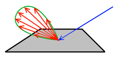
The following image will illustrate this:
You see that the blue incoming ray hits the surface and is reflected in various directions as shown by the red rays. The intensity of the transported light is depicted by a ray's length. You see that the red rays align along that green lobe. This lobe should visualize the distribution pattern of the BRDF. So, rays that are shorter transport less energy compared to longer rays.
Most surfaces that do not exhibit strong subsurface scattering can be modeled with one or the other form of BRDF. The BRDF of an actual existing matter can also be obtained empirically by shooting laser rays at it and measuring the reflected light over its hemisphere.
The easiest of such a BRDF is lambert.
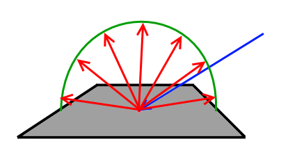
Lambertian surfaces behave in such a way that they reflect light equally in every outgoing direction, regardless of the light's incoming direction. The latter only determines how much energy the surface receives in total and therefore how much of it is reflected equally in all possible outgoing directions. The following image shows such a lambertian distribution:
Each of the red outgoing rays has the same intensity and they are distributed evenly around the hemisphere of the surface point.
This is usually how diffuse lighting works in traditional OpenGL, by the way. But there are actually very few materials in the world that behave like that.
One of those very few materials however, which has a very high diffuse reflectance over the visible spectrum, is spectralon.
The lambertian distribution property is also used to model simple light sources. A lambertian light source is therefore a light source that emits light equally in all directions.
So, now that we know the distribution of reflected light on a surface point, we can use this to decide in which direction our reflected ray is going to go. Because, whenever a ray hits a point on a surface, we must decide in which direction we want that ray to leave the surface.
With perfect mirrors it is easy to decide. We just compute the reflected ray as a function of incoming direction and surface's normal. With non-mirror-like surfaces, we have a potentially unlimited set of possible outgoing directions and should choose one direction.
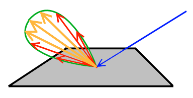
Knowing the distribution function, we choose to generate outgoing rays mainly in directions that our distribution function has the highest values. This means, given an incoming ray direction, we want to obtain those outgoing rays that transport the most energy off the surface from a given incoming ray, as shown in the following image:
Here, we would not like to waste computation energy on the red rays, which do not transport much energy off the surface, but concentrate more on tracing along the orange directions.
This approach is called Importance Sampling and, like said above, is about generating outgoing rays that transport the most light energy from the surface. This in turn helps, because we can only trace a given number of rays per unit time, so let those rays better be the ones that count in the final image!
But to actually obtain a distribution of outgoing directions, where our distribution function has the highest values for a given incoming direction, is a very non-trivial task, which is the basis of ongoing research.
Assuming, we had such a function, and knew how to sample outgoing rays for a given incoming direction on a surface point, it is very likely that this outgoing direction is not pointing to our eye. This is because we favor those outgoing directions along which the surface reflects most of the incoming light.
Knowing the distribution function of a surface, we could however generate outgoing rays that point straight at our eye. We need the distribution function then to attenuate a ray's intensity accordingly for the direction towards the eye. If that ray is not occluded by other scene geometry, this would ensure that we see our surface and we only receive that amount of light that the surface is actually reflecting in that direction.
To transport light energy not only from a surface to our eye but also between surfaces, we generate a few rays based on the distribution function to scatter some light to other surfaces as well.
So problem solved, or isn't it?
Actually not really, because there is another problem.
We try our best to make sure that rays starting from a light source and bouncing off of surfaces are eventually somehow reaching our eye.
But most of the surface points visible to our eye will actually never receive any light.
The reason for this is the distribution of the initial rays starting from the light source as well as of the few additional rays we shoot from each surface point into the scene to transport light from one surface to another.
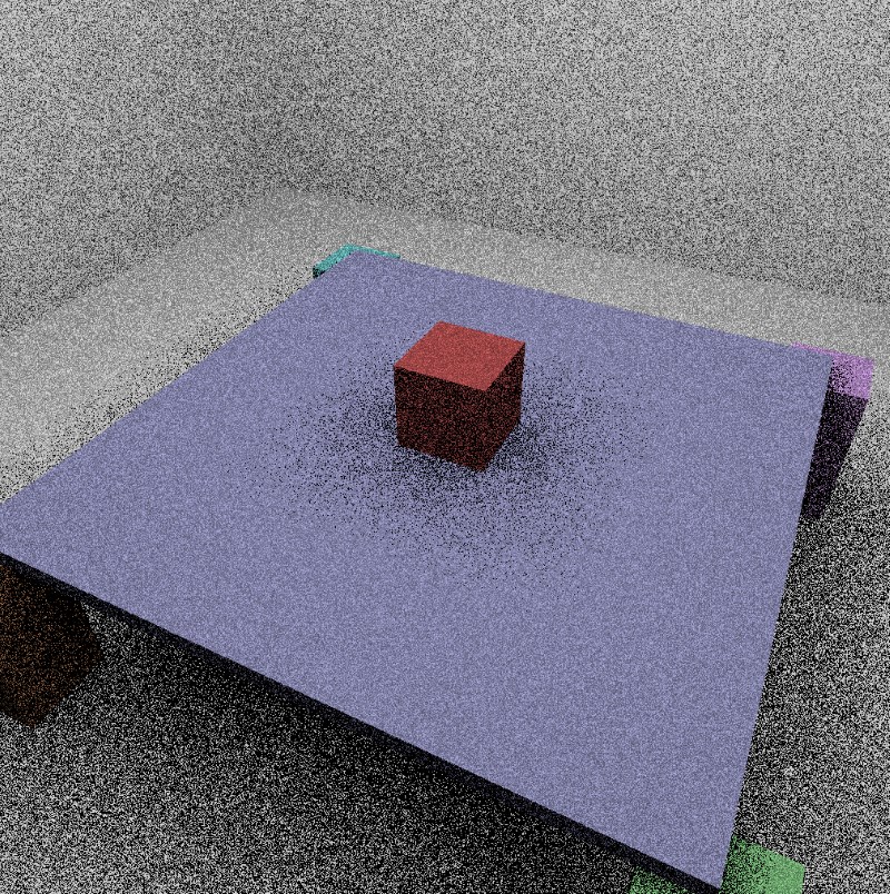
And the result of this problem will be a very grainy rendered image where certain pixels on a surface may remain completely dark whereas its neighbor pixels are bright white.
This effect is called variance, because light intensities vary quite alot at high frequencies on our rendered image, where they should not.
To be precise here, the term variance originates from the statistics branch of mathematics and describes, how much a set of numbers differ from their mean value.
Imagine those numbers to be the intensities of our pixels on the framebuffer.
When we say, the variance of our pixel's intensities is high, we usually compare those intensities to the expected/mean value, which is the physically perfect result obtained by tracing an unlimited number of rays and averaging their contributions.
When the variance is reduced and our rendered image goes towards its mean/expected value, we say that the image converges, so that the actual pixel's values and the expected values will become the same.
The following image shows the effect of variance:
So, we see that ray tracing, starting from a light source, faces serious issues. Therefore, we try to use the opposite solution, which starts with tracing rays from our eye.
When starting from the eye, we can generate rays for each of the pixels on our framebuffer/raster, make the firm assumption that eventually some light would come along this direction and then traverse those rays backwards through the scene. The path is followed to a maximum depth or until a light source is hit.
All the things said above about probability functions and importance sampling still apply here. We only swap the terms light source and eye.
When following light backwards from the eye through the scene, in addition to using importance-sampling of our distribution function to generate the reflected ray, we also generate rays that are directed towards the light sources.
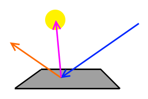
This means, whenever our ray, starting from the eye, hits a point on a surface, we generate shadow rays to all of our lights. This is illustrated by the following image:
Here, we have a yellow light source. The blue ray is the incoming light (coming from our eye) and the orange ray is the importance-sampled outgoing direction.
You see that the orange ray does not hit the light and so long this path would not transport any energy back to our eye.
We therefore generate an additional ray (the purple one), which we trace to the light.
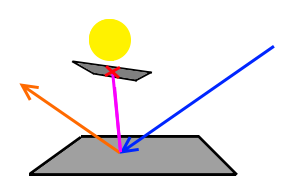
If a shadow ray intersects other scene geometry before reaching the light, that light will not contribute to the surface point's color, as is shown in the next image.
This form of ray tracing is called Path Tracing.
But if the ray makes its way to the light source, we must consult our distribution function, given that we now have two directions of light. One for the incoming light and one for the outgoing ray (to our eye).
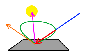
To correctly compute the light which gets reflected into our eye back along the blue ray, we therefore need to apply the distribution function to both the light direction and the incoming direction (blue). This gives us the fraction of light that is sent back the blue ray. This is depicted by the following image:
Here we can see that green lobe again, which shows the distribution of reflected light when the surface is lit by the single light source.
The distribution function has a lower value in the direction of our blue ray, so we attenuate the light's incoming energy accordingly in that direction. The resulting attenuated ray is depicted by the red ray.
After that we additionally attenuate the light's intensity by its square-distance to the surface point and the common cosine fall-off term.
This consine term you also know from OpenGL shading models, where it is simply computed as the dot-product (or inner product) of the light direction and the surface normal. That cosine fall-off term is one of the very few things in OpenGL that are actually physically correct! :-)
But this approach also has drawbacks. While rays in the first approach did not reach the eye all the time, rays in this second approach do not always reach every light source, because shadow rays can be obstructed by other scene geometry before hitting the light.
Of course, research came up with a solution for that, which is called Bidirectional Path Tracing, an algorithm published in 1993 by Eric P. Lafortune and Yves D. Willems.
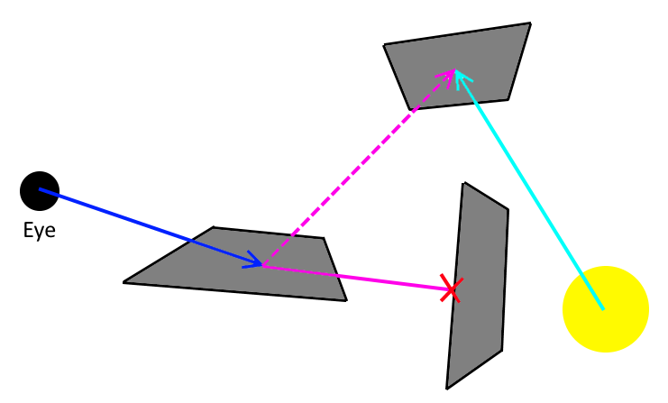
In short, this approach sends rays originating both from the eye as well as from the light sources. At each surface point hit by either of them, shadow rays are sent out to the surface hitpoints of the other, and so light paths and eye paths are connected as best as possible.
In the above image, the direct shadow ray to the light source is blocked by geometry. But since we also generated rays starting from the light source, we trace an additional shadow ray (the dotted purple ray) from the hit surface point of our eye-ray to the surface point that was hit by the light-ray. Even though the light source is not directly visible to our eye, we can still transport the optimal energy from the light to our eye.
In general however, completely solving the light transport for complex scenes is impossible to do. But this should not be a downer for us to stop even trying, because it is very well possible to achieve very realistic images in an acceptable processing time and our scenes will not have a too complex lighting situation.
You see that all approaches have their pros and cons. For our tutorial, we are going to implement a simple solution using the original Path Tracing algorithm.
Probably, you might already think "this is all good and well, but for the love of god, please show me some code!"
Okay, so here it comes. For the rest of the following text, I will however make some assumptions to keep the text as short and concise as possible.
First, you are expected to know how to build and run basic applications using LWJGL 3. This includes, how to setup JVM parameters to load the natives and such. If you feel uncomfortable with that, have a visit to the LWJGL forum. The LWJGL community will be happy to help you out on this.
I am additionally going to assume that you know how to compile shader objects and link them to a final shader program. Compute Shaders use the GL43.GL_COMPUTE_SHADER shader type for GL20.glCreateShader.
The next sections will contain GLSL code that you should be able to load, compile and link. As always, ask the community or have a look at the accompanying source code to see how to do that, if you need help on that.
We put aside most of the things said above about BRDF and importance sampling for a moment, and start with the first most simple version of our compute shader:
#version 430 core

layout(binding = 0, rgba32f) uniform image2D framebuffer;

// The camera specification
uniform vec3 eye;
uniform vec3 ray00;
uniform vec3 ray10;
uniform vec3 ray01;
uniform vec3 ray11;
This GLSL fragment declares some uniforms that our shader needs to access. You see, that the shader uses an image2D uniform, which is one level of a texture and represents our framebuffer that will be written to by our shader.
Next comes the declaration we choose for our camera, through which we view the scene.
The uniform eye will hold the camera/eye position in world-space. We do not use any projection or view transformation matrix. Instead, we will define the four corner rays of our camera's viewing frustum.
You know that in rasterization we needed to transform vertices from world-to-camera space. Now, in ray tracing we need to generate rays that we test for intersection against scene geometry.
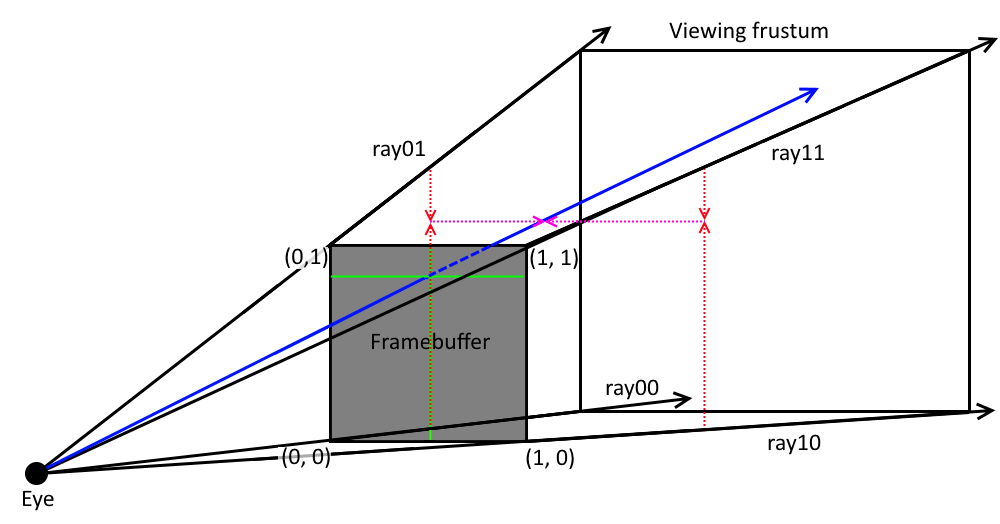
Those corner rays will span our viewing frustum along which we will interpolate to obtain a ray for each pixel in our framebuffer.
The following image shows a typical viewing frustum along with the corner rays that we use for interpolation:
On the image you see the four corner rays and the blue ray that we want to obtain via trilinear interpolation. We use the normalized framebuffer coordinates (between 0.0 and 1.0) of the framebuffer texel for which we want to generate the ray. To do that we first interpolate between the y-coordinate of ray00 and ray01 as well as ray10 and ray11. This is shown by the red dotted lines. This gives us two vectors that we interpolate along the x-coordinate to finally get the blue ray.
Technically, we obtain those corner rays by applying the inverse of the view-projection-transformation to the corner vectors of our normalized-device-coordinates system. These are (-1, -1), (+1, -1), (-1, +1) and (+1, +1). In order to not compute that complicated matrix transformation for every pixel, we instead compute the corner rays in the host program and interpolate between them in our shader.
Compared to rasterization, ray tracing allows us to define other types of primitives than just triangles.
For our simple demo application, we will be using axis-aligned boxes. Such a box can be defined by its min-corner and max-corner coordinates, both as three-dimensional vectors. So we continue our GLSL code from the previous listing with:
struct box {
  vec3 min;
  vec3 max;
};

#define NUM_BOXES 2
const box boxes[] = {
  /* The ground */
  {vec3(-5.0, -0.1, -5.0), vec3(5.0, 0.0, 5.0)},
  /* Box in the middle */
  {vec3(-0.5, 0.0, -0.5), vec3(0.5, 1.0, 0.5)}
};
Here, we define a ground plate which is a thin box ranging from -5 to +5 in X and Z dimension and whose base position should be Y = 0.
After that, we define a small box standing at the center of our ground plate.
We could just as well use triangles to be able to render triangle meshes, but for the sake of simplicity, we stick to boxes, also because testing rays against axis-aligned boxes for intersection is quite simple:
vec2 intersectBox(vec3 origin, vec3 dir, const box b) {
  vec3 tMin = (b.min - origin) / dir;
  vec3 tMax = (b.max - origin) / dir;
  vec3 t1 = min(tMin, tMax);
  vec3 t2 = max(tMin, tMax);
  float tNear = max(max(t1.x, t1.y), t1.z);
  float tFar = min(min(t2.x, t2.y), t2.z);
  return vec2(tNear, tFar);
}
Using the parametric form of a ray, which is origin + t * dir, the above function returns the t at which the ray enters the given box. Additionally, it also returns the far intersection, at which the ray exits the box. If the ray does not hit the box, the far value will be less than the near value. And if the box lies behind the ray, the near value will be negative.
The following image shows a ray intersecting a box:
Here, the near intersection parameter value is t1 and the far intersection parameter is t2.
The final test whether the ray actually hit the box will be:
vec2 lambda = intersectBox(...);
bool hit = lambda.x > 0.0 && lambda.x < lambda.y;
We not only want to test our ray against a single box, but instead against our whole scene:
#define MAX_SCENE_BOUNDS 1000.0

struct hitinfo {
  vec2 lambda;
  int bi;
};

bool intersectBoxes(vec3 origin, vec3 dir, out hitinfo info) {
  float smallest = MAX_SCENE_BOUNDS;
  bool found = false;
  for (int i = 0; i < NUM_BOXES; i++) {
    vec2 lambda = intersectBox(origin, dir, boxes[i]);
    if (lambda.x > 0.0 && lambda.x < lambda.y && lambda.x < smallest) {
      info.lambda = lambda;
      info.bi = i;
      smallest = lambda.x;
      found = true;
    }
  }
  return found;
}
This function computes the nearest intersection of the given ray with all of our boxes in the scene.
Additionally, the hitinfo struct is used to return (as out-parameter) the hit position and the index of the box that was hit, because we need that information later.
Now, that we can test a ray against all of our objects in the scene and receive the information about the closest hit, we can use that intersectBoxes function in a simple way:
vec4 trace(vec3 origin, vec3 dir) {
  hitinfo i;
  if (intersectBoxes(origin, dir, i)) {
    vec4 gray = vec4(i.bi / 10.0 + 0.8);
    return vec4(gray.rgb, 1.0);
  }
  return vec4(0.0, 0.0, 0.0, 1.0);
}
The responsibility of this function is to return the amount of light that a given ray contributes when perceived by our eye.
So, any ray that we use as input will originate from our eye and go through the framebuffer texel that we are currently computing in the shader invocation.
For the first version of this function, this function just traces the given ray into the scene and returns some gray scale if a box was hit, or returns black if nothing was hit.
Like all other shader stages, a Compute Shader also needs a main function, that gets called when our shader is invoked by the GPU:
layout (local_size_x = 8, local_size_y = 8) in;

void main(void) {
  ivec2 pix = ivec2(gl_GlobalInvocationID.xy);
  ivec2 size = imageSize(framebuffer);
  if (pix.x >= size.x || pix.y >= size.y) {
    return;
  }
  vec2 pos = vec2(pix) / vec2(size.x, size.y);
  vec3 dir = mix(mix(ray00, ray01, pos.y), mix(ray10, ray11, pos.y), pos.x);
  vec4 color = trace(eye, dir);
  imageStore(framebuffer, pix, color);
}
Here, we first obtain our shader invocation's ID, which is stored in the predefined gl_GlobalInvocationID. This gives the position of our shader invocation in terms of the previously mentioned three-dimensional integer range, which is the domain of a Compute Shader. So, we need to know where in that integer range we are with a particular shader invocation.
We naturally define that the x-coordinate of the invocation ID is the x-coordinate of our framebuffer's texel that we want to compute. The same goes for the y-coordinate.
With this information, we check whether our shader invocation is within the bounds of our framebuffer, which is obtained via the GLSL function imageSize. It is explained later why bounds checking is necessary. We will also get to know what that layout declaration is all about.
After bounds checking, we compute the ray from our eye through the current pixel via trilinear interpolation of the viewing frustum's corner rays via the GLSL mix function.
As interpolation weight factors, we simply use the invocation ID of the shader divided by our framebuffer size in each dimension.
Lastly, we call our trace function and write the returned value into our framebuffer using the GLSL imageStore function, which takes an image, two integer texel coordinates (as ivec2) and the value/color to write.
That last step is essentially what a fragment shader does implicitly when used together with a framebuffer object (FBO) to which a texture is attached.
Here you see where the parallels between the OpenGL rasterization API and the Compute Shaders are. Compute Shaders just offer a closer-to-the-metal view of things and allow to mix-and-match computation and memory accesses as you wish. You could even have multiple render targets (MRT) support by not just writing to a single image but writing different values to multiple different images in the Compute Shader.
In the last sections, we rushed through the GLSL Compute Shader code to obtain a working version. Now we need to setup OpenGL and create some resources in our host program to use that shader.
I will however assume that you know how to create OpenGL textures, vertex array objects (VAO), vertex buffer objects (VBO) and shader objects and programs.
Therefore, I will just use pseudocode to illustrate what needs to be done and whether anything special needs to be taken care of:
void initialization() {
  int tex = create new texture object

  setup min/mag NEAR filtering for that texture
  initialize texture as 2D rgba32f FLOAT and some width/height

  int vao = create VertexArrayObject of full-screen-quad
  // This quad is used to render our
  // "framebuffer" texture onto the screen.

  int computeProgram = create-and-link program with single compute shader object

  int quadProgram = create-and-link simple full-screen quad vertex and fragment shader
  // The fragment shader would fetch
  // texels from our "tex" texture.

  Setup constant uniforms in quad program, such as "tex" texture unit = 0
}
In the code above we create four OpenGL objects:
- One texture, which will serve as our framebuffer with RGBA32F format
- One VAO which simply holds our full-screen-quad to present the framebuffer texture once it is generated by our ray tracing shader
- Our ray tracing Compute Shader
- and our quad shader to render the full-screen quad VAO with the framebuffer as texture
Notice, that we are using a single-precision floating point format for our framebuffer texture. This is explained in the next part of the tutorial when we are going to accumulate and average multiple frames together.
The rendering process to produce one frame will be as follows:
- Bind the Compute Shader
- Setup camera properties in compute shader uniforms
- Bind level 0 of framebuffer texture to image binding point 0
- Start/dispatch the compute shader to generate a frame in the framebuffer image
- Unbind image binding point
- Bind the written framebuffer texture in OpenGL to texture unit 0
- Bind the full-screen shader program
- Bind the full-screen-quad VAO
- Draw the VAO
- Release all bindings
There are two things that need thorough explanation:
- How do we bind an image of a texture to a Compute Shader
- How do we invoke a Compute Shader
The first is accomplished via GL42.glBindImageTexture. It introduces a new image binding point in OpenGL that a shader uses to read and write a single level of a texture and that we will bind the first level of our framebuffer texture to.
Invoking a shader is as simple as calling GL43.glDispatchCompute. This function takes as argument the number of work groups in each of the three possible dimensions. The number of work groups is NOT the number of global work items in each dimension, but is divided by the work group size that the shader specified in that layout declaration.
We want to have exactly as many shader invocations as our framebuffer has pixels in width and height.
The layout of our domain will be:
- the first dimension of the shader domain will map to the U/X-axis of our framebuffer image
- the second dimension of the shader domain will map to the V/Y-axis of our framebuffer image
To see how we create that number of invocations in both dimensions we must first understand what that layout declaration in the shader was all about.
Like CUDA and OpenCL, the OpenGL Compute Shader execution model is also centered around work groups.
All invocations/threads running inside the same work group can use shared memory and can be synchronized. This is a feature that is not exposed in any other OpenGL shader stages and allows us to build efficient algorithms in an OpenGL Compute Shader.
So, that layout declaration specifies the size of a work group (in number of work items for each dimension), which must be a power of two.
And since GL43.glDispatchCompute takes the number of work groups as parameters, we must compute how many work groups we need in order to cover our whole computation (our framebuffer).
To do that, we first query the shader program for its declared work group size using GL20.glGetProgram with GL43.GL_COMPUTE_WORK_GROUP_SIZE and then we divide our required number of computations (i.e. work items) by that value.
We only have one problem, though: Our framebuffer size need not be a power of two, but both our work group size as well as the number of work groups must be.
So, after dividing the framebuffer size by the work group size, we must round up that number to its next power of two.
You can do that with this nifty function found at bits.stephan-brumme.com:
static int nextPowerOfTwo(int x) {
  x--;
  x |= x >> 1; // handle 2 bit numbers
  x |= x >> 2; // handle 4 bit numbers
  x |= x >> 4; // handle 8 bit numbers
  x |= x >> 8; // handle 16 bit numbers
  x |= x >> 16; // handle 32 bit numbers
  x++;
  return x;
}In this section we will discuss how to obtain the viewing frustum's corner rays that our shader needs in order to compute the correct ray for each framebuffer texel.
First, it is convenient and common to have some sort of matrix representation of your camera-to-world transformation.
Usually, this is done by a 4x4 matrix and is separated into a perspective projection matrix and a view matrix.
Since we are not using legacy OpenGL with its matrix stacks anymore, we have to roll our own camera transformations.
To do that, you first need to have some linear algebra support on matrices and vectors in your application. The accompanying example code uses gwt-vecmath for this, which itself is a fork of the Java3D's popular vecmath library.
Second, it is useful to have a class representing your camera in terms of its position, its up vector and its viewing direction.
With this information, you would generate a view transformation matrix.
If you want to know how to do that, have a look at OpenGL Projection Matrix.
You would additionally need a way to generate a perspective projection matrix based on field-of-view and ratio. This is also layed out in the mentioned web article.
To spare you the trouble, all of those things are already taken care of by the class "Camera" in the accompanying source code, which you can freely use in your code.
Just like with gluPerspective and gluLookAt, you can configure your projection and view transformations and obtain the corresponding transformations as 4x4 matrices.
Now, that we have linear algebra and a camera representation settled, we can compute the corner rays of our viewing frustum like so:
mat4x4 invViewProjMat = (viewMat * projMat)^(-1)
ray00 = (-1, -1, 0, 1) * invViewProjMat
ray00 /= ray00.w
ray00 -= camera.position
ray10 = (+1, -1, 0, 1) * invViewProjMat
ray10 /= ray10.w
ray10 -= camera.position
// accordingly for ray01 and ray11
We first compute the inverse, denoted by the ^(-1), of the combined view-projection-matrix.
This will allow us to convert from clipping space to world space.
Using this matrix, we transform our corner vectors (given as -1, +1 in X and Y), perform perspective-divide and subtract the camera's position.
For the first start, we setup our camera using these parameters:
position = (3.0, 2.0, 7.0)
up = (0.0, 1.0, 0.0)
lookat = (0.0, 0.5, 0.0)
fov = 60.0
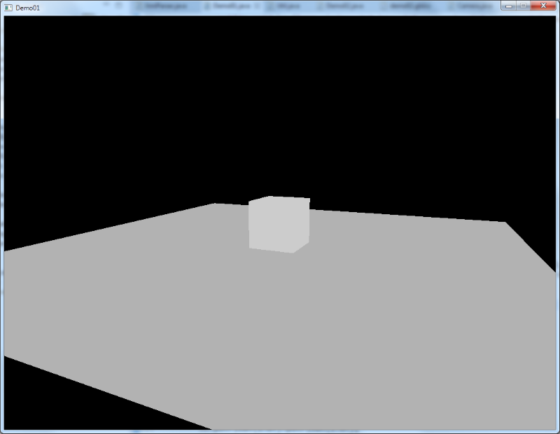
ratio = (framebuffer width / height)If you coded all this down or just used the accompanying code example and run it, you should see something like this:
Probably, you wonder why we went through all that trouble to render a simple ground plate and a cube sitting on it that is all gray and boring. "Where are the shadows and where is that global illumination that you praised so much before", you might wonder. :-)
Well, since this post is now really getting too long, I will postpone that to the next one.
There, we will add lighting that fits this scene as well as use multisampling antialiasing with distributed ray tracing.
This article provided the ground work to augment this simple demo application with all sorts of technical things, like shader subroutines to define multiple materials as shader functions and activate/select them as needed.
Other things on the horizon include correct depth-of-field simulation by integrating over our camera's aperture.
I have all of this already down in GLSL and Java. Just the tutorial text needs to be written and edited and some illustrations prepared! :-)
So, stay tuned!
In the end, things will look like this:
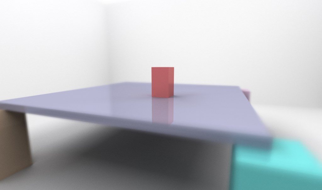
You see that with very little code we have built ourselves a fine ray tracer. Admittedly, it cannot render a general scene yet, comprising of triangle meshes. But it shows where the differences between rasterization and ray tracing are.
With rasterization, we would throw triangles through our transformations and onto the screen, where they are processes one after the other and generate fragments whose attributes we can store somewhere, such as the color and depth on the framebuffer or on some texture for deferred shading.
With ray tracing, we have to have an explicit or implicit description of the whole scene at any time accessible to the Compute Shader. We use this description then to query the scene for intersections with rays.
This first simple demo application performs very well on hardware supporting Compute Shaders. There are two reasons for that. First, our scene description is very simple, consisting of only two boxes. And second, we only trace the first ray from the eye into the scene. That could also have been achieved easily with standard rasterization.
In the next part, we will see that things change very rapidly, when we both increase the number of objects in our scene as well as the number of bounces we follow our rays along.
We will also begin to notice that in the future some optimizations may be required in order to remain at realtime framerates, as we trace more and more rays through our scene for various effects.
If you liked all that and are now all psyched up to get to know more, I highly recommend you to get a copy of the following two excellent books:
- Real Time Rendering, 3rd Edition by Tomas Akenine-Moller, Eric Haines and Naty Hoffman
- Physically Based Rendering, 2nd Edition by Matt Pharr and Greg Humphreys
Hey, I am Kai Burjack, simply known as "Kai" in the forum. I am living in Hamburg, Germany where I am employed as an IT consultant. Since 2008, I have been using LWJGL during my Master degree studies of Computer Science in Media and also for hobby projects. It wasn't until recently that I am also using LWJGL in a customer project, which is about path tracing.
