MortalityTables

A Julia package for working with MortalityTables. Has:

• Lots of bundled SOA mort.soa.org tables
• survivorship and cumualtive_decrement functions to calculate decrements over period of time
• Partial year mortality calculations (Uniform, Constant, Balducci)
• Friendly syntax and flexible usage

Examples

Quickstart

Loading the package and bundled tables:

julia> using MortalityTables

julia> tables = MortalityTables.tables()
Dict{String,MortalityTable} with 266 entries:
  "2015 VBT Female Non-Smoker RR90 ALB"                                       => SelectUltimateTable{OffsetArray{OffsetArray{Float64,1,Array{Float64,1}},1,Array{OffsetArray{F…  
  "2017 Loaded CSO Preferred Structure Nonsmoker Preferred Female ANB"        => SelectUltimateTable{OffsetArray{OffsetArray{Float64,1,Array{Float64,1}},1,Array{OffsetArray{F…  
  ⋮                                                                            => ⋮

Get information about a particular table:

julia> vbt2001 = tables["2001 VBT Residual Standard Select and Ultimate - Male Nonsmoker, ANB"]
MortalityTable (Insured Lives Mortality):
   Name:
       2001 VBT Residual Standard Select and Ultimate - Male Nonsmoker, ANB
   Fields:
       (:select, :ultimate, :metadata)
   Provider:
       Society of Actuaries
   mort.SOA.org ID:
       1118
   mort.SOA.org link:
       https://mort.soa.org/ViewTable.aspx?&TableIdentity=1118
   Description:
       2001 Valuation Basic Table (VBT) Residual Standard Select and Ultimate Table -  Male Nonsmoker.
       Basis: Age Nearest Birthday. 
       Minimum Select Age: 0. 
       Maximum Select Age: 99. 
       Minimum Ultimate Age: 25. 
       Maximum Ultimate Age: 120

The package revolves around easy-to-access vectors which are indexed by attained age:

julia> vbt2001.select[35] # vector of rates for issue age 35
 0.00036
 0.00048
 ⋮
 0.94729
 1.0
julia> vbt2001.select[35][35] #issue age 35, attained age 35

julia> vbt2001.ultimate[95]  # ultimate vectors only need to be called with the attained age
0.24298

Calculate the force of mortality or survivorship over a range of time:

julia> survivorship(vbt2001.ultimate,30,40) # the survivorship between ages 30 and 40
0.9894404665434904

julia> decrement(vbt2001.ultimate,30,40) # the decrement between ages 30 and 40
0.010559533456509618

Non-whole periods of time are supported when you specify the assumption (Constant(), Uniform(), or Balducci()) for fractional periods:

julia> survivorship(vbt2001.ultimate,30,40.5,Uniform()) # the survivorship between ages 30 and 40.5
0.9887676470262408

Example: Quickly access and compare tables

using MortalityTables, Plots


tables = MortalityTables.tables()
cso_2001 = tables["2001 CSO Super Preferred Select and Ultimate - Male Nonsmoker, ANB"]
cso_2017 = tables["2017 Loaded CSO Preferred Structure Nonsmoker Super Preferred Male ANB"]

issue_age = 27
durations = 1:30
mort = [
     cso_2001.select[issue_age][issue_age .+ durations .- 1],
     cso_2017.select[issue_age][issue_age .+ durations .- 1],
     ]
plot(
   durations,
   mort,
   label = ["2001 CSO" "2017 CSO"],
   title = "Comparison of 2107 and 2001 CSO \n for SuperPref NS 27-year-old male",
   xlabel="duration")

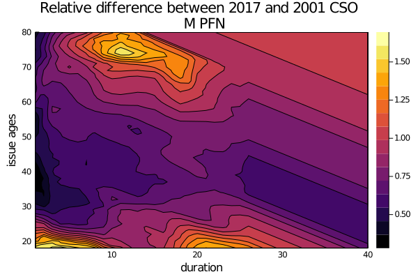
Easily extend the analysis to move up the ladder of abstraction:

issue_ages = 18:80
durations = 1:40

# compute the relative rates with the element-wise division ("brodcasting" in Julia)
function rel_diff(a, b, issue_age,duration)
        att_age = issue_age + duration - 1
        return a[issue_age][att_age] / b[issue_age][att_age]
end


diff = [rel_diff(cso_2017.select,cso_2001.select,ia,dur) for ia in issue_ages, dur in durations]
contour(durations,
        issue_ages,
        diff,
        xlabel="duration",ylabel="issue ages",
        title="Relative difference between 2017 and 2001 CSO \n M PFN",
        fill=true
        )

Example: Scaling and capping a table

Say that you want to take a given mortality table, scale it by 130%, and cap it at 1.0. You can do this easliy by broadcasting over the underlying rates (which is really just a vector of numbers at the end of the day):

issue_age = 30
m = cso_2001.select[issue_age]

scaled_m = min.(cso_2001.select[issue_age] .* 1.3, 1.0) # 130% and capped at 1.0 version of `m`

Note that min.(cso_2001.select .* 1.3, 1.0) won't work because cso_2001.select is still a vector-of-vectors (a vector for each issue age). You need to drill down to a given issue age or use an ulitmate table to manipulate the rates in this way.

Fractional Years

When evaluating survival over partial years when you are given full year mortality rates, you must make an assumption over how those deaths are distributed throughout the year. Three assumptions are provided as options and are based on formulas from the 2016 Experience Study Calculations paper from the SOA, specifically pages 40-44.

The three assumptions are:

• Uniform() which assumes an increasing force of mortality throughout the year.
• Constant() which assumes a level force of mortality throughout the year.
• Balducci() which assumes a decreasing force of mortality over the year. It seems to be for making it easier to calculate successive months by hand.

Some Batteries Included

Comes with some tables built in via mort.SOA.org and by using you agree to their terms.

Not all tables have been tested that they work by default, though no issues have been reported with any of the the VBT/CSO/other common tables.

Sample of some of the included table sets:

2017 Loaded CSO
2015 VBT
2001 VBT
2001 CSO
1980 CSO
1980 CET

Click here to see the full list of tables included.

Parameterized Models

Makeham and Gompertz's Law is included. Use like so:

a = 0.00022
b = 2.7e-6
c = 1.124
m = Makeham(a,b,c)
g = Gompertz(b,c)

Now some examples with m, but could use g interchangably:

age = 20
m[20] # the mortality rate at age 20
decrement(m,20,25) # the five year cumulative mortality rate
survivorship(m,20,25) # the five year survivorship rate

Adding more tables

Getting tables from mort.SOA.org

Given a table id (for example 60029) you can request the table directly from the SOA's mortality table service. Remember that not all tables have been tested, though the standard source format should mean compatibility with MortalityTables.jl.

aus_life_table_female = get_SOA_table(60029)
aus_life_table_female[0]  # returns the attained age 0 rate of 0.10139

You can combine it with the bundled tables too:

tables = MortalityTables.tables()

get_SOA_table!(tables,60029) # this modifies `tables` by adding the new table

t = tables["Australian Life Tables 1891-1900 Female"]
t[0]  # returns the attained age 0 rate of 0.10139

Constructing Dynamically

Say you have an ultimate vector and select matrix, and you want to leverage the MortalityTables package.

Here's an example, where we first construct the UlitmateMortality and then combine it with the select rates to get a SelectMortality table.

using MortalityTables

# represents attained ages of 15 through 100
ult_vec = [0.005, 0.008, ...,0.805,1.00]
ult = UltimateMortality(ult_vec,start_age = 15)

We can now use this the ulitmate rates all by itself:

q(ult,15,1) # 0.005

And join with the select rates, which for our example will start at age 0:

# attained age going down the column, duration across
select_matrix = [ 0.001 0.002 ... 0.010;
                  0.002 0.003 ... 0.012;
                  ...
                ]
sel_start_age = 0
sel = SelectMortality(select_matrix,ult,start_age = 0)

sel[0][0] #issue age 0, attained age 0 rate of  0.001
sel[0][100] #issue age 0, attained age 100 rate of  1.0

Lastly, to take the SelectMortality and UltimateMortality we just created, we can combine them into one stored object, along with a TableMetaData:

my_table = MortalityTable(
              s1,
              u1,
              metadata=TableMetaData(name="My Table", comments="Rates for Product XYZ")
              )

Load with bundled tables

To add more tables for your use when loading with all of the other bundled tables, download the .xml aka the (XTbML format) version of the table from mort.SOA.org and place it in the directory the package is installed in. This is usually ~user/.julia/packages/MortalityTables/[changing hash value]/src/tables/.

⚠️ updating the package may remove your existing tables. Make a backup before updating your packages

After placing packages in the folder above, restart Julia and the should be discoverable when you run mt.Tables()

Getting more tables bundled with the package

If you would like more tables added by default, please open a GitHub issue with the request.

References

• SOA Mortality Tables
• Actuarial Mathematics for Life Contingent Risks, 2nd ed
• Experience Study Calculations, SOA

Similar Projects

• Pyliferisk, a Python package