#The Fast Bilateral Solver (Still in development)

The Bilater Solver is a novel algorithm for edge-aware smoothing that combines the flexibility and speed of simple filtering approaches with the accuracy of domain-specific optimization algorithms. This algorithm was presented by Jonathan T. Barron and Ben Poole as an ECCV2016 oral and best paper nominee. Algorithm details and applications can be found in https://arxiv.org/pdf/1511.03296.pdf .

---

[TOC]

---

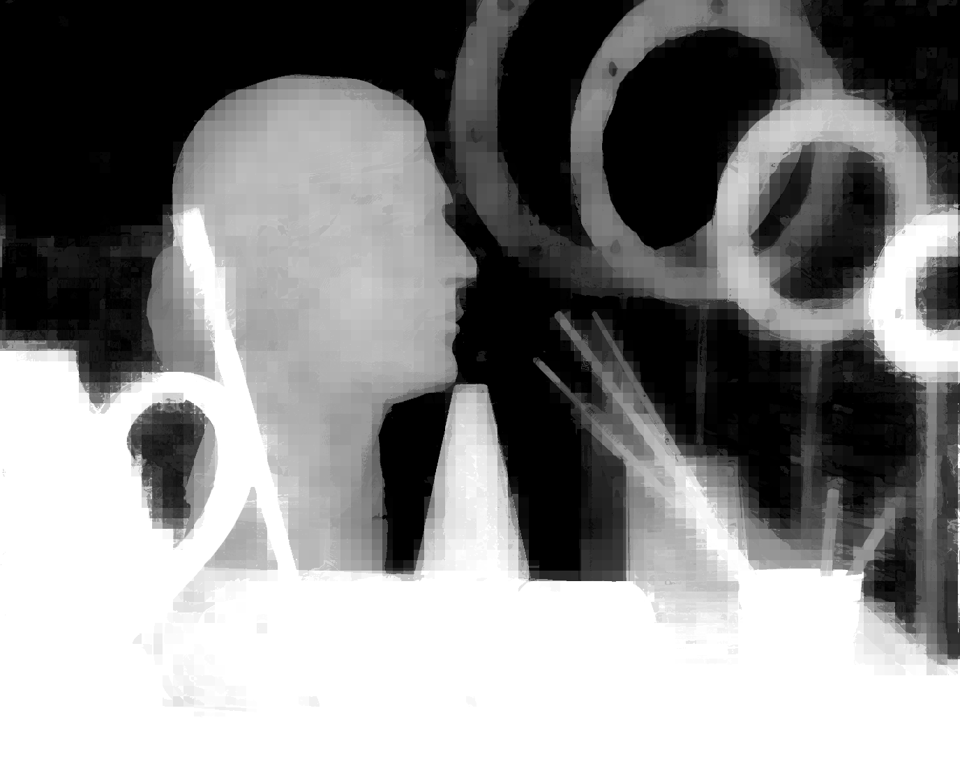
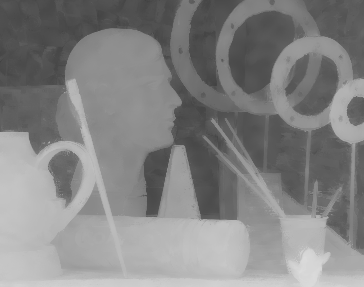
##Introduce ###Algorithm We begin by presenting the objective and optimization techniques that make up our bilateral solver. Let us assume that we have some per-pixel input quantities t (the “target” value, see Figure 1a) and some per-pixel confidence of those quantities c (Figure 1c), both represented as vectorized images. Let us also assume that we have some “reference” image (Figure 1d), which is a normal RGB image. Our goal is to recover an “output” vector x (Figure 1b), which will resemble the input target where the confidence is large while being smooth and tightly aligned to edges in the reference image. We will accomplish this by constructing an optimization problem consisting of an image-dependent smoothness term that encourages x to be bilateral-smooth, and a data-fidelity term that minimizes the squared residual between x and the target t weighted by our confidence c: $$minimize\frac{\lambda}{2}\sum_{i,j}\widehat{W}{i,j}(x_i-x_j)^{2}+\sum{i}(c_i-t_i)^{2} \quad (1)$$ The smoothness term in this optimization problem is built around an affinity matrix Ŵ , which is a bistochastized version of a bilateral affinity matrix W . Each element of the bilateral affinity matrix $W_{i,j}$ reflects the affinity between pixels i and j in the reference image in the YUV colorspace: $$W_{i,j} = \exp(-\frac{\left |[p_i^x,p_i^y]-[[p_j^x,p_j^y]]\right |}{2\sigma_{xy}^2}-\frac{(p_i^l-p_j^l)^2}{2\sigma_{l}^2}-\frac{\left |[p_i^u,p_i^v]-[[p_j^u,p_j^v]]\right |}{2\sigma_{uv}^2})\quad (2)$$ Where $p_i$ is a pixel in our reference image with a spatial position $(p_i^x, p_i^y )$ and color $(p_i^l , p_i^u , p_i^v )$. The $\sigma_{xy} , \sigma_l$ , and $σ_{uv}$ parameters control the extent of the spatial, luma, and chroma support of the filter, respectively. This W matrix is commonly used in the bilateral filter, an edge-preserving filter that blurs within regions but not across edges by locally adapting the filter to the image content. There are techniques for speeding up bilateral filtering which treat the filter as a “splat/blur/slice” procedure: pixel values are “splatted” onto a small set of vertices in a grid or lattice (a soft histogramming operation), then those vertex values are blurred, and then the filtered pixel values are produced via a “slice” (an interpolation) of the blurred vertex values. These splat/blur/slice filtering approaches all correspond to a compact and efficient factorization of W : $$W = S^T\overline{B}S\quad (3)$$ Barron et al. built on this idea to allow for optimization problems to be “splatted” and solved in bilateral-space. They use a “simplified” bilateral grid and a technique for producing bistochastization matrices $D_n , D_m$ that together give the the following equivalences: $$\widehat{W} = S^TD_m^{-1}D_n\overline{B}D_nD_m^{-1}S , SS^T = D_m\quad (4)$$ They also perform a variable substitution, which reformulates a high-dimensional pixel-space optimization problem in terms of the lower-dimensional bilateral-space vertices: $$x = S^Ty\quad (5)$$ Where y is a small vector of values for each bilateral-space vertex, while x is a large vector of values for each pixel. With these tools we can not only reformulate our pixel-space loss function in Eq 1 in bilateral-space, but we can rewrite that bilateral-space loss function in a quadratic form: $$minimize\frac{1}{2}y^TAy - b^Ty + c\quad (6)$$ $$A = \lambda(D_m - D_n\overline{B}D_n) + diag(S\textbf c)$$ $$b = S(\textbf c \circ \textbf t)$$ $$c = \frac{1}{2}(\textbf c \circ \textbf t)^T\textbf t$$ where $\circ$ is the Hadamard product. A derivation of this reformulation can be found in the supplement. While the optimization problem in Equation 1 is intractably expensive to solve naively, in this bilateral-space formulation optimization can be performed quickly. Minimizing that quadratic form is equivalent to solving a sparse linear system: $$Ay = b\quad (7)$$ We can produce a pixel-space solution x̂ by simply slicing the solution to that linear system: $$\widehat{x} = S^T(A^{-1}b) \quad (8)$$ With this we can describe our algorithm, which we will refer to as the “bilateral solver.” The input to the solver is a reference RGB image, a target image that contains noisy observed quantities which we wish to improve, and a confidence image. We construct a simplified bilateral grid from the reference image, which is bistochastized as in [2] (see the supplement for details), and with that we construct the A matrix and b vector described in Equation 6 which are used to solve the linear system in Equation 8 to produce an output image. If we have multiple target images (with the same reference and confidence images) then we can construct a larger linear system in which b has many columns, and solve for each channel simultaneously using the same A matrix. In this many-target case, if b is low rank then that property can be exploited to accelerate optimization, as we show in the supplement.

###Implementation

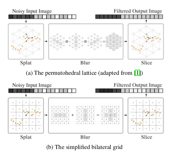
• Splat+Blur+Slice Procedure The two bilateral representations we use in this project, here shown filtering a toy one-dimensional grayscale image of a step-edge. This toy image corresponds to a 2D space visualized here (x = pixel location, y = pixel value) while in the paper we use RGB images, which corresponds to a 5D space (XYRGB). The lattice (Fig 2a) uses barycen-tric interpolation to map pixels to vertices and requires d+1 blurring operations, where d is the dimensionality of the space. The simplified bilateral grid (Fig 2b) uses nearest-neighbor interpolation and requires d blurring operations which are summed rather than done in sequence. The grid is cheaper to construct and to use than the lattice, but the use of hard assignments means that the filtered output often has blocky piecewise-constant artifacts.

• Diagrammatize

st=>start: Start
e=>end

inr=>operation: Imput reference image
int=>operation: Imput target image
bg=>operation: construct BilateralGrid
sl=>operation: construct SliceMatrix
bl=>operation: construct BlurMatrix
A1=>operation: construct AMatrix step1
A2=>operation: construct AMatrix step2
cg=>operation: execute ICCG
out=>operation: output the resolt


st->inr->bg->sl->bl->A1->int->A2->cg->out->e

###Reference

article{BarronPoole2016,
author = {Jonathan T Barron and Ben Poole},
title = {The Fast Bilateral Solver},
journal = {ECCV},
year = {2016},
}
@article{Barron2015A,
author = {Jonathan T Barron and Andrew Adams and YiChang Shih and Carlos Hern\'andez},
title = {Fast Bilateral-Space Stereo for Synthetic Defocus},
journal = {CVPR},
year = {2015},
}
@article{Adams2010,
author = {Andrew Adams	Jongmin Baek	Abe Davis},
title = {Fast High-Dimensional Filtering Using the Permutohedral Lattice},
journal = {Eurographics},
year = {2010},
}

---

##Installation Instructions

Build OpenCV

This is just a suggestion on how to build OpenCV 3.1. There a plenty of options. Also some packages might be optional.

sudo apt-get install libgtk2.0-dev pkg-config libavcodec-dev libavformat-dev libswscale-dev python-dev python-numpy libtbb2 libtbb-dev libjpeg-dev libpng-dev libtiff-dev libjasper-dev libdc1394-22-dev
git clone https://github.com/Itseez/opencv.git
cd opencv
mkdir build
cd build
cmake -D CMAKE_BUILD_TYPE=RELEASE -D WITH_CUDA=OFF ..
make -j
sudo make install

#notice :

if you have build failure with this error : unsupported/Eigen/MatrixFunctions: No such file or directory.

You have to find the path of unsupported/Eigen/MatrixFunctions. In my case it was inside /usr/include/eigen3/.

Then to solve the problem you have to open modules/contrib/src/rgbdodometry.cpp and add "eigen3/" to the include path at line 65.

###Build The_Bilateral_Solver

git clone https://github.com/THUKey/The_Bilateral_Solver.git
cd The_Bilateral_Solver/build
cmake ..
make

This will create three executable demos, that you can run as shown in below.

####Depthsuperresolution

the target.

./Depthsuperres

This result(use bilateral solver) is far from the optimal performance, which means there are some extra work to do, such as to patiently adjustment parameters and to optimize the implementation.

./Latticefilter reference.png target.png

This result(use permutohedral_lattice) is quite nice. ####Colorization

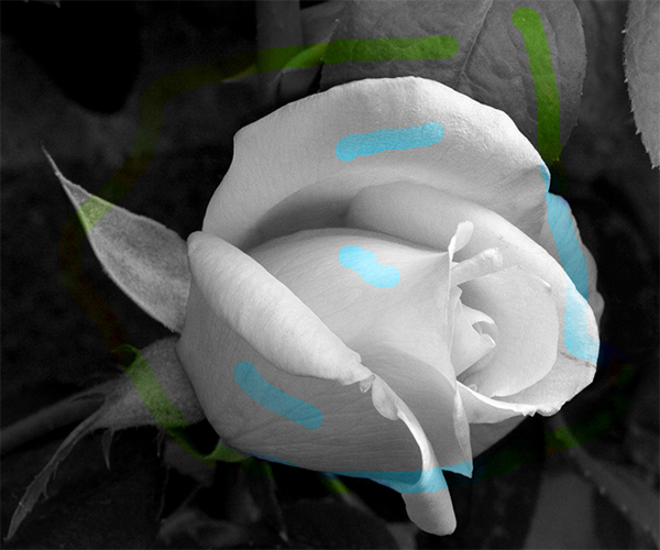
./Colorize rose1.webp

draw image, then press "ESC" twice to launch the colorization procession. colorized image. you could change the rose1.webp to your own image. Thanks for timuda, his colorization implementation help me a lot.

####PermutohedralLatticeFilter

./Latticefilter flower8.jpg

In Barron's another paper Fast Bilateral-Space Stereo for Synthetic Defocus, both bileteral_solver and permutohedral lattice are used to do experiment, and the result shows that bilateral_solver is faster than permutohedral lattice technique, but the permutohedral is more accurate than the bilateral_solver. In other words, this is the tradeoff between time and accuracy. Actually, both two techniques' tradeoff can be worthwhile in appropriate condition. So I want to implement both two technique for more widely use. filter_output. filter_input.

---

##Basic Usage

Depthsuperresolution:

	BilateralGrid BiGr(mat_R);
	BiGr.Depthsuperresolution(mat_R,mat_T,sigma_spatial,sigma_luma,sigma_chroma);

Firstly, we use the reference image mat_R construct a BilateralGrid, the we launch a depthsuperresolution to optimize the target image mat_T. The parameter sigma_spatial is the Gaussian kernal for coordinate x y, similarly , the sigma_luma correspond luma(Y) and the sigma_chroma correspond chroma(UV). It need to be noted that he mat_R should be covert to YUV form before construct the bilateralgrid.

###Colorization

	InputImage InImg(mat_in);
	mat_bg_in = InImg.get_Image(IMG_YUV);
	InImg.draw_Image();
	mat_bg_draw_in = InImg.get_Image(IMG_DRAWYUV);
	BilateralGrid BiGr(mat_bg_in);
	BiGr.Colorization(mat_in,mat_bg_draw_in);

Similar to above, we need to covert the imput image mat_in(gray image for colorization) to YUV form, then draw the gray image. when the drawing finished, press "ESC" twice to launch the colorization procession. the result will be save in specified folder. ###PermutohedralLattce

	bilateral(im,spatialSigma,colorSigma);

Similar to BilateralGrid, the PermutohedralLattce also need spatial parameter and the color parameter to specified the Gaussian kernel.

---

##Schedule

Item	State	Remark
C++ code of the core algorithm	Completed	also python
Depthsuperres module	Completed	need optimize
Colorization module	Completed	choose ICCG or others
PermutohedralLatticeFilter	Completed	increse Compatibility
Semantic Segmentation optimizer	Ongoing	try apply in CNN
Contribute project to OpenCV	Ongoing	coding testfile
Detail Documentation	Ongoing	writing toturial