random_points
A common need in distribution modeling is to randomly sample a multi-dimensional regular grid. Random sampling is required when using presence-only models (like maxent). You may need to avoid missing data, presence points, or confine your search to a polygon.
twinkle provides the random_points() function to generate random
points. Let’s load the three Penobscot Bay datasets, an associated
polygon.
We load all of the data, but we’ll actually just take the first 2 days of the month to keep things simple.
suppressPackageStartupMessages(
  { library(stars)
    library(sf)
    library(twinkle)
  }
)

x <- list(
  stars::read_stars(system.file("datasets/20140601-20140630-sst.tif",
                                     package = "twinkle"))[,,,1:2],
  stars::read_stars(system.file("datasets/20140601-20140630-sst_slope.tif",
                                       package = "twinkle"))[,,,1:2],
  stars::read_stars(system.file("datasets/20140601-20140630-sst_cum.tif",
                                       package = "twinkle"))[,,,1:2] ) |>
  bind_attrs() |>
  rlang::set_names(c("sst", "slope", "cum")) |>
  stars::st_set_dimensions("band",
                           names = "date",
                           point = TRUE,
                           values = as.Date(c("2014-06-01", "2014-06-02")))

poly <- sf::read_sf(system.file("datasets/penbay-polygons.gpkg", package = 'twinkle'))First we can simply sample everywhere. We’ll show the points draped over just the bands for the first attribute (in this case ‘sst’).
rnd_pts <- random_points(x)
par(mfrow = c(1,2))
i <- 1
plot(x[1,,,i], reset = FALSE, key.pos = NULL,
   main = paste("sst", i),
   add.geom = list(sf::st_geometry(dplyr::filter(rnd_pts, band == i)),
                   col = "orange", pch = 19))
i <- 2
plot(x[1,,,i], reset = FALSE, key.pos = NULL,
   main = paste("sst", i),
   add.geom = list(sf::st_geometry(dplyr::filter(rnd_pts, band == i)),
                   col = "olivedrab", pch = 19))
par(mfrow = c(1,1))Let’s look at the contents of the random points (see below). In addition to the data values (sst, slope and cum) at each point, we also retrieve some simple navigation information about each point.
- geometry in this case 2d POINT at cell centers,
- index a three dimensional index to the col/row/band location,
- cell a 2 dimensional index to each cell within a band,
- col/row row and column indices,
- band the band index number (not the band value).
rnd_pts
# Simple feature collection with 100 features and 8 fields
# geometry type:  POINT
# dimension:      XY
# bbox:           xmin: -69.19 ymin: 43.79 xmax: -68.49 ymax: 44.5
# geographic CRS: WGS 84
# # A tibble: 100 x 9
#    index  cell   col   row  band   sst      slope    cum       geometry
#    <int> <dbl> <dbl> <dbl> <dbl> <dbl>      <dbl>  <dbl>    <POINT [°]>
#  1  5709   597    29     9     2  282.  0.0000266 42333. (-68.91 44.42)
#  2  5430   318    34     5     2  282. NA         42328. (-68.86 44.46)
#  3  9859  4747    61    67     2  282.  0.0000340 42573. (-68.59 43.84)
#  4  4933  4933    34    70     1  282.  0.0000100 42226. (-68.86 43.81)
#  5  1388  1388    39    20     1   NA  NA            NA  (-68.81 44.31)
#  6  6913  1801    26    26     2  283.  0.0000151 42356. (-68.94 44.25)
#  7  8046  2934    23    42     2  283.  0.0000215 42385. (-68.97 44.09)
#  8  2612  2612    56    37     1  283.  0.0000492 42130. (-68.64 44.14)
#  9 10146  5034    64    71     2  282.  0.0000348 42599.  (-68.56 43.8)
# 10  6421  1309    31    19     2  283.  0.0000232 42350. (-68.89 44.32)
# # … with 90 more rows
rnd_pts <- random_points(x, na.rm = TRUE)
par(mfrow = c(1,2))
i <- 1
plot(x[1,,,i], reset = FALSE, key.pos = NULL,
   main = paste("sst", i),
   add.geom = list(sf::st_geometry(dplyr::filter(rnd_pts, band == i)),
                   col = "orange", pch = 19))
i <- 2
plot(x[1,,,i], reset = FALSE, key.pos = NULL,
   main = paste("sst", i),
   add.geom = list(sf::st_geometry(dplyr::filter(rnd_pts, band == i)),
                   col = "olivedrab", pch = 19))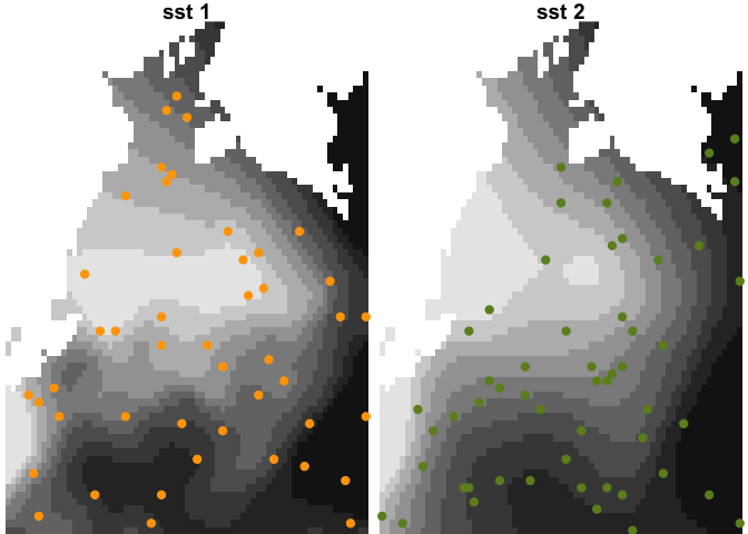
par(mfrow = c(1,1))We suppress messages only because we get this
although coordinates are longitude/latitude, st_contains assumes that they are planar
At this scale it probably doesn’t matter.
suppressMessages(rnd_pts <- random_points(x, n = 50, polygon = poly))
par(mfrow = c(1,2))
i <- 1
plot(x[1,,,i], reset = FALSE, key.pos = NULL,
   main = paste("sst", i),
   add.geom = list(sf::st_geometry(dplyr::filter(rnd_pts, band == i)),
                   col = "orange", pch = 19))
plot(poly, add = TRUE, border = "pink", color = NA)

i <- 2
plot(x[1,,,i], reset = FALSE, key.pos = NULL,
   main = paste("sst", i),
   add.geom = list(sf::st_geometry(dplyr::filter(rnd_pts, band == i)),
                   col = "olivedrab", pch = 19))
plot(poly, add = TRUE, border = "pink", color = NA)
par(mfrow = c(1,1))We generate some points to avoid; note that we rename the ‘band’
variable to be ‘date’ to match the band name in x.
avoid_pts <- random_points(x, n = 50, polygon = poly) |>
  dplyr::rename(date = band)
pts <- random_points(x, n = 100, points = avoid_pts, polygon  = poly)

par(mfrow = c(1,2))
i <- 1
plot(x[1,,,i], reset = FALSE, key.pos = NULL,
   main = paste("sst", i),
   add.geom = list(sf::st_geometry(dplyr::filter(pts, band == i)),
                   col = "orange", pch = 19))
plot(sf::st_geometry(poly), add = TRUE, border = "pink", col = NA)
plot(sf::st_geometry(dplyr::filter(avoid_pts, date == i)), add = TRUE,
     pch = 0, col = "steelblue")

i <- 2
plot(x[1,,,i], reset = FALSE, key.pos = NULL,
   main = paste("sst", i),
   add.geom = list(sf::st_geometry(dplyr::filter(rnd_pts, band == i)),
                   col = "olivedrab", pch = 19))
plot(sf::st_geometry(poly), add = TRUE, border = "pink", col = NA)
plot(sf::st_geometry(dplyr::filter(avoid_pts, date == i)), add = TRUE,
     pch = 0, col = "yellow")
par(mfrow = c(1,1))As shown above, you can specify a combination of polygons to search
within, points to avoid, and na.rm. The order of operation is…
-
select n*m points at random either at large or within
polygonif provided, -
remove NAs if
na.rm = TRUE, -
avoid specified points is
!is.null(points)Note that it’s actually cells to avoid as identified by the specified points.