A toolkit to evaluate neural network explanations

PyTorch and Tensorflow

Quantus is currently under active development so carefully note the Quantus release version to ensure reproducibility of your work.

📑 Shortcut to paper!

News and Highlights! 🚀

• Please see our latest release which minor version includes some heavy API changes!
• Offers more than 30+ metrics in 6 categories for XAI evaluation
• Supports different data types (image, time-series, NLP next up!) and models (PyTorch and Tensorflow)
• Latest metrics additions:
  • Infidelity (Chih-Kuan, Yeh, et al., 2019)
  • ROAD (Rong, Leemann, et al., 2022)
  • Focus (Arias et al., 2022)
  • Consistency (Dasgupta et al., 2022)
  • Sufficiency (Dasgupta et al., 2022)
• New optimisations added: BatchedMetric and BatchedPerturbationMetric help to speed up evaluation computation!

Citation

If you find this toolkit or its companion paper Quantus: An Explainable AI Toolkit for Responsible Evaluation of Neural Network Explanations interesting or useful in your research, use following Bibtex annotation to cite us:

@article{hedstrom2022quantus,
      title={Quantus: An Explainable AI Toolkit for Responsible Evaluation of Neural Network Explanations}, 
      author={Anna Hedström and
              Leander Weber and
              Dilyara Bareeva and
              Franz Motzkus and
              Wojciech Samek and
              Sebastian Lapuschkin and
              Marina M.-C. Höhne},
      year={2022},
      eprint={2202.06861},
      archivePrefix={arXiv},
      primaryClass={cs.LG}
}

When applying the individual metrics of Quantus, please make sure to also properly cite the work of the original authors (as linked above).

Table of contents

• Library overview
• Installation
• Getting started
• Tutorials
• Misc functionality
• Contributing

Library overview

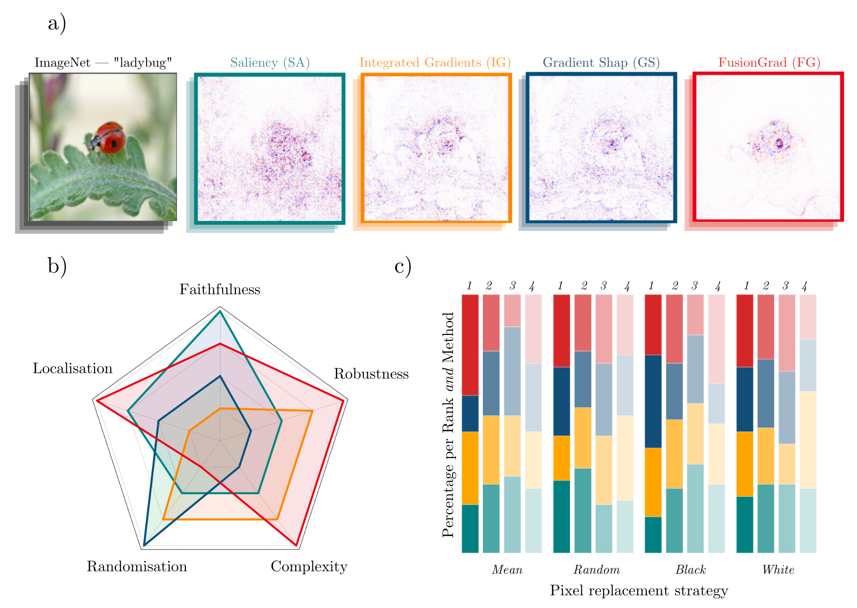
Simple visual comparison of eXplainable Artificial Intelligence (XAI) methods is often not sufficient to decide which explanation method works best as shown exemplary in Figure a) for four gradient-based methods — Saliency (Mørch et al., 1995; Baehrens et al., 2010), Integrated Gradients (Sundararajan et al., 2017), GradientShap (Lundberg and Lee, 2017) or FusionGrad (Bykov et al., 2021), yet it is a common practice for evaluation XAI methods in absence of ground truth data.

Therefore, we developed Quantus, an easy to-use yet comprehensive toolbox for quantitative evaluation of explanations — including 30+ different metrics. With Quantus, we can obtain richer insights on how the methods compare e.g., b) by holistic quantification on several evaluation criteria and c) by providing sensitivity analysis of how a single parameter e.g. the pixel replacement strategy of a faithfulness test influences the ranking of the XAI methods.

This project started with the goal of collecting existing evaluation metrics that have been introduced in the context of XAI research — to help automate the task of XAI quantification. Along the way of implementation, it became clear that XAI metrics most often belong to one out of six categories i.e., 1) faithfulness, 2) robustness, 3) localisation 4) complexity 5) randomisation or 6) axiomatic metrics (note, however, that the categories are oftentimes mentioned under different naming conventions e.g., 'robustness' is often replaced for 'stability' or 'sensitivity' and 'faithfulness' is commonly interchanged for 'fidelity'). The library contains implementations of the following evaluation metrics:

Faithfulness

quantifies to what extent explanations follow the predictive behaviour of the model (asserting that more important features play a larger role in model outcomes)

• Faithfulness Correlation (Bhatt et al., 2020): iteratively replaces a random subset of given attributions with a baseline value and then measuring the correlation between the sum of this attribution subset and the difference in function output
• Faithfulness Estimate (Alvarez-Melis et al., 2018): computes the correlation between probability drops and attribution scores on various points
• Monotonicity Metric (Arya et al. 2019): starts from a reference baseline to then incrementally replace each feature in a sorted attribution vector, measuring the effect on model performance
• Monotonicity Metric (Nguyen et al, 2020): measures the spearman rank correlation between the absolute values of the attribution and the uncertainty in the probability estimation
• Pixel Flipping (Bach et al., 2015): captures the impact of perturbing pixels in descending order according to the attributed value on the classification score
• Region Perturbation (Samek et al., 2015): is an extension of Pixel-Flipping to flip an area rather than a single pixel
• Selectivity (Montavon et al., 2018): measures how quickly an evaluated prediction function starts to drop when removing features with the highest attributed values
• SensitivityN (Ancona et al., 2019): computes the correlation between the sum of the attributions and the variation in the target output while varying the fraction of the total number of features, averaged over several test samples
• IROF (Rieger at el., 2020): computes the area over the curve per class for sorted mean importances of feature segments (superpixels) as they are iteratively removed (and prediction scores are collected), averaged over several test samples
• Infidelity (Chih-Kuan, Yeh, et al., 2019): represents the expected mean square error between 1) a dot product of an attribution and input perturbation and 2) difference in model output after significant perturbation
• ROAD (Rong, Leemann, et al., 2022): measures the accuracy of the model on the test set in an iterative process of removing k most important pixels, at each step k most relevant pixels (MoRF order) are replaced with noisy linear imputations
• Sufficiency (Dasgupta et al., 2022): measures the extent to which similar explanations have the same prediction label

Robustness

measures to what extent explanations are stable when subject to slight perturbations of the input, assuming that model output approximately stayed the same

• Local Lipschitz Estimate (Alvarez-Melis et al., 2018): tests the consistency in the explanation between adjacent examples
• Max-Sensitivity (Yeh et al., 2019): measures the maximum sensitivity of an explanation using a Monte Carlo sampling-based approximation
• Avg-Sensitivity (Yeh et al., 2019): measures the average sensitivity of an explanation using a Monte Carlo sampling-based approximation
• Continuity (Montavon et al., 2018): captures the strongest variation in explanation of an input and its perturbed version
• Consistency (Dasgupta et al., 2022): measures the probability that the inputs with the same explanation have the same prediction label

Localisation

tests if the explainable evidence is centered around a region of interest (RoI) which may be defined around an object by a bounding box, a segmentation mask or, a cell within a grid

• Pointing Game (Zhang et al., 2018): checks whether attribution with the highest score is located within the targeted object
• Attribution Localization (Kohlbrenner et al., 2020): measures the ratio of positive attributions within the targeted object towards the total positive attributions
• Top-K Intersection (Theiner et al., 2021): computes the intersection between a ground truth mask and the binarized explanation at the top k feature locations
• Relevance Rank Accuracy (Arras et al., 2021): measures the ratio of highly attributed pixels within a ground-truth mask towards the size of the ground truth mask
• Relevance Mass Accuracy (Arras et al., 2021): measures the ratio of positively attributed attributions inside the ground-truth mask towards the overall positive attributions
• AUC (Fawcett et al., 2006): compares the ranking between attributions and a given ground-truth mask
• Focus (Arias et al., 2022): quantifies the precision of the explanation by creating mosaics of data instances from different classes

Complexity

captures to what extent explanations are concise i.e., that few features are used to explain a model prediction

• Sparseness (Chalasani et al., 2020): uses the Gini Index for measuring, if only highly attributed features are truly predictive of the model output
• Complexity (Bhatt et al., 2020): computes the entropy of the fractional contribution of all features to the total magnitude of the attribution individually
• Effective Complexity (Nguyen at el., 2020): measures how many attributions in absolute values are exceeding a certain threshold

Randomisation

tests to what extent explanations deteriorate as inputs to the evaluation problem e.g., model parameters are increasingly randomised

• Model Parameter Randomisation (Adebayo et. al., 2018): randomises the parameters of single model layers in a cascading or independent way and measures the distance of the respective explanation to the original explanation
• Random Logit Test (Sixt et al., 2020): computes for the distance between the original explanation and the explanation for a random other class

Axiomatic

assesses if explanations fulfill certain axiomatic properties

• Completeness (Sundararajan et al., 2017): evaluates whether the sum of attributions is equal to the difference between the function values at the input x and baseline x'.
• Non-Sensitivity (Nguyen at el., 2020): measures whether the total attribution is proportional to the explainable evidence at the model output (and referred to as Summation to Delta (Shrikumar et al., 2017), Sensitivity-n (slight variation, Ancona et al., 2018) and Conservation (Montavon et al., 2018))
• Input Invariance (Kindermans et al., 2017): adds a shift to input, asking that attributions should not change in response (assuming the model does not)

Additional metrics will be included in future releases.

Disclaimers. It is worth noting that the implementations of the metrics in this library have not been verified by the original authors. Thus any metric implementation in this library may differ from the original authors. Further, bear in mind that evaluation metrics for XAI methods are often empirical interpretations (or translations) of qualities that some researcher(s) claimed were important for explanations to fulfill, so it may be a discrepancy between what the author claims to measure by the proposed metric and what is actually measured e.g., using entropy as an operationalisation of explanation complexity.

The first iteration has been developed primarily for image classification tasks, with attribution-based explanations in mind (which is a category of explanation methods that aim to assign an importance value to the model features and arguably, is the most studied kind of explanation). As a result, there will be both applications and explanation methods e.g., example-based methods where this library won't be applicable. Similarly, there is a couple of metrics that are popular but are considered out of scope for the first iteration of the library e.g., metrics that require re-training of the network e.g., RoAR (Hooker et al., 2018) and Label Randomisation Test (Adebayo et al., 2018) or rely on specifically designed datasets/ dataset modification e.g., Model Contrast Scores and Input Dependence Rate (Yang et al., 2019) and Attribution Percentage (Attr%) (Zhou et al., 2021).

Please read the user guidelines for further guidance on how to best use the library.

Installation

Installing from PyPI

If you already have PyTorch or Tensorflow installed on your machine, the most light-weight version of Quantus can be obtained from PyPI as follows (i.e., this means that additional explainability functionality, as well as ML frameworks will not be included):

pip install quantus

Alternatively, you can simply add the desired framework (in brackets), and it will be installed in addition to Quantus: For PyTorch:

pip install "quantus[torch]"

For Tensorflow:

pip install "quantus[tensorflow]"

Installing from requirements.txt

Alternatively, you can simply install from the requirements.txt found here, however, this only installs with the default setup, requiring either PyTorch or Tensorflow:

pip install -r requirements.txt

Installing XAI Library Support (PyPI only)

Most evaluation metrics in Quantus allow for a choice of either providing pre-computed explanations directly as an input, or to instead make use of several wrappers implemented in quantus.explain around common explainability libraries. The following XAI Libraries are currently supported:

Captum

To enable the use of wrappers around Captum, you can run:

pip install "quantus[captum]"

tf-explain

To enable the use of wrappers around tf.explain, you can run:

pip install "quantus[tf-explain]"

Zennit

To use Quantus with support for the Zennit library, you can run:

pip install "quantus[zennit]"

Note that the three options above will also install the respective required frameworks (i.e., PyTorch or Tensorflow), if they are not already installed in your environment.

Installing Tutorial Requirements

The Quantus tutorials have more requirements than the base package, which you can install by running

pip install "quantus[tutorials]"

Full Installation

To simply install all of the above, you can run

pip install "quantus[full]"

Package Requirements

The package requirments are as follows:

python>=3.7.0
pytorch>=1.10.1
tensorflow==2.6.2
tqdm==4.62.3

Getting started

The following will give a short introduction for how to get started with Quantus.

Note: This example is based on the PyTorch framework, but we also support Tensorflow, which would differ only in the {ref}preliminaries <prelim> (i.e., the model and data loading), as well as in the available XAI libraries.

Preliminaries

(prelim)= Quantus implements methods for the quantitative evaluation of XAI methods. Generally, in order to apply these, you will need:

• A model (variable model)
• Input data and labels (variables x_batch and y_batch)
• Explanations to evaluate (variables a_batch_*)

Model and Data

Let's first load the model and the data. In this example, a pre-trained LeNet available from Quantus for the purpose of this tutorial is loaded, but generally you might use any Pytorch (or Tensorflow) model instead.

import quantus
from quantus import LeNet
import torch
import torchvision

# Enable GPU.
device = torch.device("cuda:0" if torch.cuda.is_available() else "cpu")

# Load a pre-trained LeNet classification model (architecture at quantus/helpers/models).
model = LeNet()
model.load_state_dict(torch.load("tests/assets/mnist_model"))

# Load datasets and make loaders.
test_set = torchvision.datasets.MNIST(root='./sample_data', download=True)
test_loader = torch.utils.data.DataLoader(test_set, batch_size=24)

# Load a batch of inputs and outputs to use for XAI evaluation.
x_batch, y_batch = iter(test_loader).next()
x_batch, y_batch = x_batch.cpu().numpy(), y_batch.cpu().numpy()

Explanations

We still need some explanations to evaluate. For this, there are two possibilities in Quantus:

Using Pre-computed Explanations

Quantus allows you to evaluate explanations that you have already computed previously, assuming that they match the data you provide in x_batch. Let's say you have explanations for Saliency and Integrated Gradients already pre-computed.

In that case, you can simply load these into corresponding variables a_batch_saliency and a_batch_intgrad:

a_batch_saliency = load("path/to/precomputed/saliency/explanations")
a_batch_saliency = load("path/to/precomputed/intgrad/explanations")

Using Quantus XAI Wrappers

The second possibility (if you don't have the explanations you are interested in available already) is to simply obtain them from one of the many XAI frameworks out there, such as Captum, Zennit, tf.explain, or iNNvestigate.

The following code example shows how to obtain explanations (Saliency and Integrated Gradients, to be specific) using Captum:

import captum
from captum.attr import Saliency, IntegratedGradients

# Generate Integrated Gradients attributions of the first batch of the test set.
a_batch_saliency = Saliency(model).attribute(inputs=x_batch, target=y_batch, abs=True).sum(axis=1).cpu().numpy()
a_batch_intgrad = IntegratedGradients(model).attribute(inputs=x_batch, target=y_batch, baselines=torch.zeros_like(x_batch)).sum(axis=1).cpu().numpy()

# Save x_batch and y_batch as numpy arrays that will be used to call metric instances.
x_batch, y_batch = x_batch.cpu().numpy(), y_batch.cpu().numpy()

# Quick assert.
assert [isinstance(obj, np.ndarray) for obj in [x_batch, y_batch, a_batch_saliency, a_batch_intgrad]]

# You can use any function (not necessarily captum) to generate your explanations.

However, this can be tedious if you want to compare multiple explanation methods, or switch hyperparameters, or even the XAI library used to compute explanations. For these reasons, the quantus.explain function offers wrappers around Captum, Zennit, and tf.explain, so that explanations do not need to be computed by hand as shown above, and complex evaluations can be performed using less code.

The qualitative aspects of explanations may look fairly uninterpretable - since we lack ground truth of what the explanations should be looking like, it is hard to draw conclusions about the explainable evidence that we see:

So, to quantitatively evaluate the explanations, we can apply Quantus.

Evaluating Explanations with Quantus

Quantus Metrics

Quantus implements XAI evaluation metrics from different categories (faithfulness, localisation, robustness, ...) which all inherit from the base quantus.Metric class. Metrics are designed as Callables. To apply a metric to your setting (e.g., Max-Sensitivity), they first need to be instantiated:

max_sensitivity = quantus.MaxSensitivity()

and then applied to your model, data, and (pre-computed) explanations:

result = max_sensitivity(
    model=model,
    x_batch=x_batch,
    y_batch=y_batch,
    a_batch=a_batch_salicency,
    device=device
)

Alternatively, if you want to employ the quantus.explain utility instead of pre-computing explanations, you can call the metric like this:

result = max_sensitivity(
    model=model,
    x_batch=x_batch,
    y_batch=y_batch,
    device=device,
    explain_func=quantus.explain,
    explain_func_kwargs={"method": "Saliency"})
)

Customising Metrics

The metrics for evaluating XAI methods are often quite sensitive to their respective hyperparameters. For instance, how explanations are normalised or whether signed or unsigned explanations are considered can have significant impact on the results of the evaluation. However, some metrics require normalisation or unsigned values, while others are more flexible.

Therefore, different metrics can have different hyperparameters or default values in Quantus, which are documented in detail {doc}here </docs_api/modules>. We encourage users to read the respective documentation before applying each metric, to gain an understanding of the implications of altering each hyperparameter.

Nevertheless, for the purpose of robust evaluation, it makes sense to vary especially those hyperparameters that metrics tend to be sensitive to. Generally, hyperparameters for each metric are separated as follows:

• Hyperparameters affecting the metric function itself are set in the __init__ method of each metric. Extending the above example of MaxSensitivity, various init hyperparameters can be set as follows:

  max_sensitivity = quantus.MaxSensitivity(
      nr_samples=10,
      lower_bound=0.2,
      norm_numerator=quantus.fro_norm,
      norm_denominator=quantus.fro_norm,
      perturb_func=quantus.uniform_noise,
      similarity_func=quantus.difference
  )
• Hyperparameters affecting the inputs (data, model, explanations) to each metric are set in the __call__ method of each metric. Extending the above example of MaxSensitivity, various call hyperparameters can be set as follows:

  result = max_sensitivity(
      model=model,
      x_batch=x_batch,
      y_batch=y_batch,
      device=device,
      explain_func=quantus.explain,
      explain_func_kwargs={"method": "Saliency"},
      softmax=False
  )

Large-Scale Evaluations

Quantus also provides high-level functionality to support large-scale evaluations, e.g., multiple XAI methods, multifaceted evaluation through several metrics, or a combination thereof.

To utilize quantus.evaluate(), you simply need to define two dictionaries:

• The XAI Methods you would like to evaluate:

  xai_methods = {
      "Saliency": a_batch_saliency,
      "IntegratedGradients": a_batch_intgrad
  }
• The Metrics you would like to use for evaluation (each __init__ parameter configuration counts as its own metric):

  metrics = {
      "max-sensitivity-10": quantus.MaxSensitivity(nr_samples=10),
      "max-sensitivity-20": quantus.MaxSensitivity(nr_samples=20),
      "region-perturbation": quantus.RegionPerturbation(),
  }

After defining how to aggregate the measurements of each metric on each XAI-method, you can then simply run a large-scale evaluation as

import numpy as np

agg_func = np.mean
metric_call_kwargs = {
  "model"=model,
  "x_batch"=x_batch,
  "y_batch"=y_batch,
  "softmax": False,
}

results = quantus.evaluate(
      metrics=metrics,
      xai_methods=xai_methods,
      agg_func=np.mean,
      **metric_call_kwargs
)

You can find a dedicated notebook similar to the example in this tutorial here: Getting started.

Extending Quantus

With Quantus, one can flexibly extend the library's functionality, e.g., to adopt a customised explainer function explain_func or to replace a function that perturbs the input perturb_func with a user-defined one. If you are extending or replacing a function within the Quantus framework, make sure that your new function:

• has the same return type
• expects the same arguments

as the function you’re intending to replace.

Details on what datatypes and arguments that should be used for the different functions can be found in the respective function typing in {doc}quantus.helpers</docs_api/quantus.helpers>. For example, if you want to replace similarity_func in your evaluation, you can do as follows.

import scipy
import numpy as np

def my_similarity_func(a: np.array, b: np.array, **kwargs) -> float:
    """Calculate the similarity of a and b by subtraction."""
    return a - b

# Simply initalise the metric with your own function.
metric = quantus.LocalLipschitzEstimate(similarity_func=my_similar_func)

Similarly, if you are replacing or extending metrics, make sure they inherit from the Metric class in {doc}quantus.metrics.base</docs_api/quantus.metrics.base>. Each metric at least needs to implement the Metric.evaluate_instance method.

Miscellaneous

There are several miscellaneous helpers built-into Quantus intended for easier usability:

# Interpret scores of a given metric.
metric_instance.interpret_scores

# Understand the hyperparameters of a metric.
sensitivity_scorer.get_params

# To list available metrics (and their corresponding categories).
quantus.AVAILABLE_METRICS

# To list available explainable methods.
quantus.AVAILABLE_XAI_METHODS

# To list available perturbation functions.
quantus.AVAILABLE_SIMILARITY_FUNCTIONS

# To list available similarity functions.
quantus.AVAILABLE_PERTURBATION_FUNCTIONS

# To list available normalisation function.
quantus.AVAILABLE_NORMALISATION_FUNCTIONS

# To get the scores of the last evaluated batch.
metric_instance_called.last_results

Per default, warnings are printed to shell with each metric initialisation in order to make the user attentive to the hyperparameters of the metric which may have great influence on the evaluation outcome. If you are running evaluation iteratively you might want to disable warnings, then set:

disable_warnings = True

in the params of the metric initalisation. Additionally, if you want to track progress while evaluating your explanations set:

display_progressbar = True

If you want to return an aggreagate score for your test samples you can set the following hyperparameter:

return_aggregate = True

for which you can specify an aggregate_func e.g., np.mean to use while aggregating the score for a given metric.

Tutorials

Further tutorials are available that showcase the many types of analysis that can be done using Quantus. For this purpose, please see notebooks in tutorials folder which includes examples such as:

• ImageNet Example All Metrics: shows how to instantiate the different metrics for ImageNet
• Metric Parameterisation Analysis: explores how sensitive a metric could be to its hyperparameters
• Explanation Sensitivity Evaluation Model Training: looks into how robustness of gradient-based explanations change as model gets increasingly accurate in its predictions
• ImageNet Quantification with Quantus: benchmarks explanation methods under different types of analysis: qualitative, quantitative and sensitivity ... and more.

Contributing

We welcome any sort of contribution to Quantus. For a detailed contribution guide, please refer to Contributing documentation first.