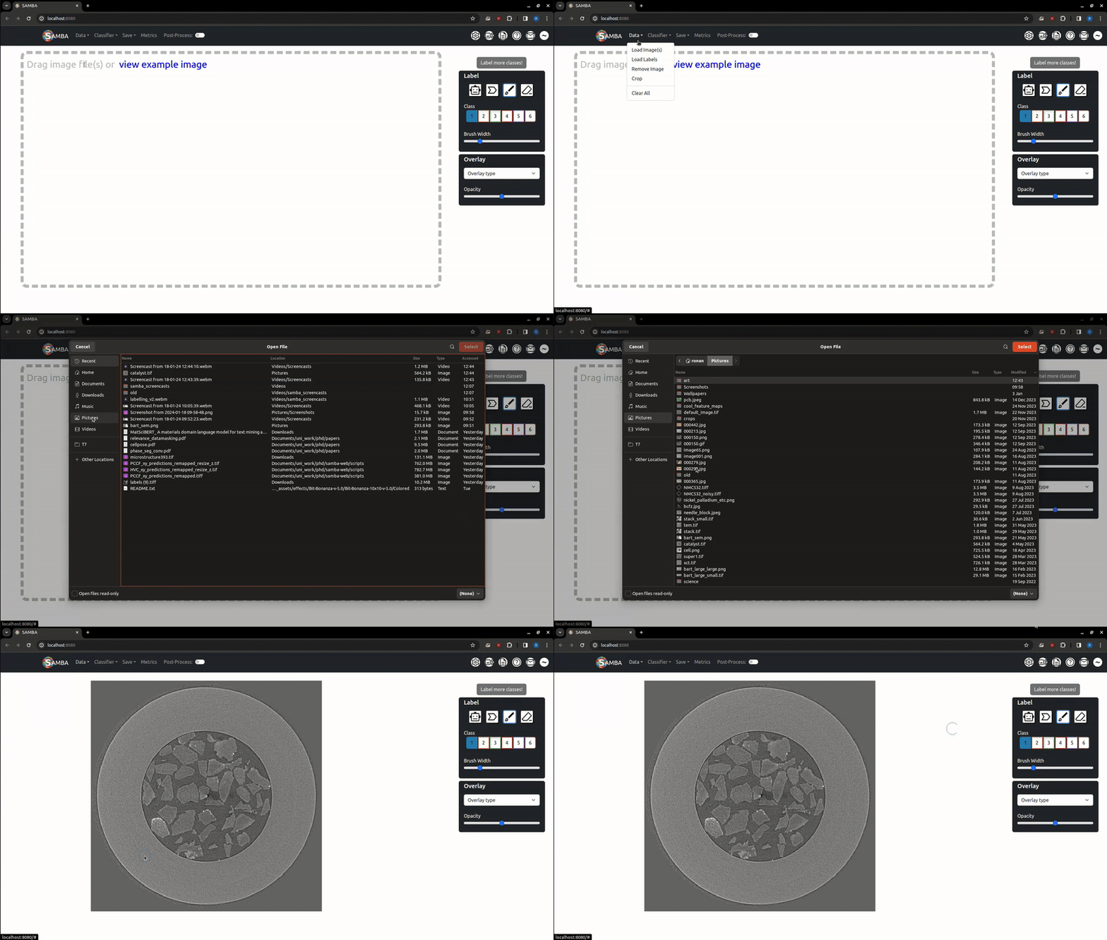
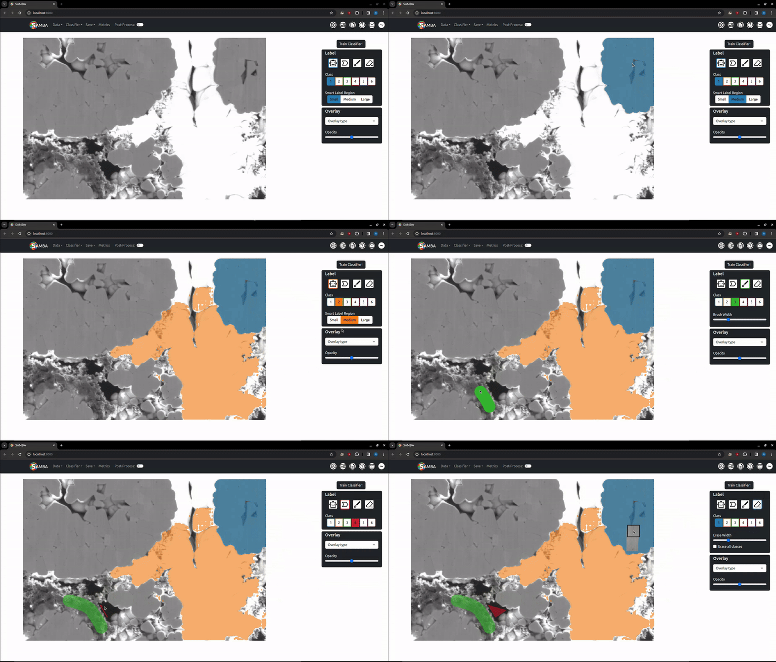
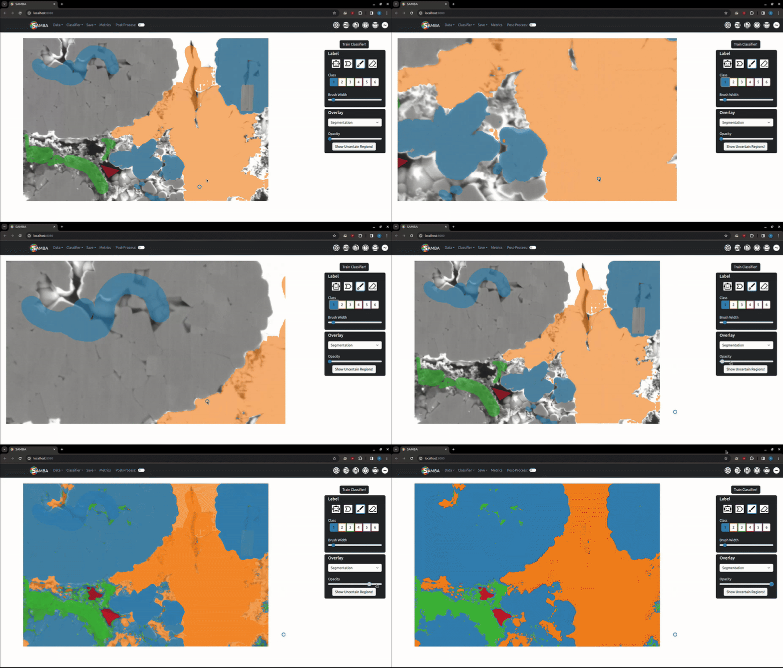
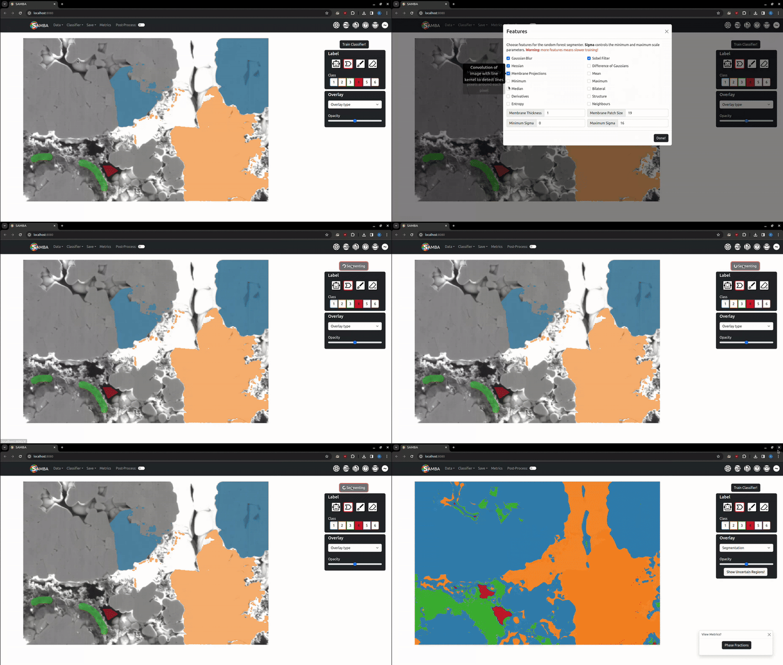
A video tutorial is also available.
Click the 'Add' button in the 'Data' dropdown or drag and drop an image file. Accepted types are .jpg. .png and .tiff. The image cannot be larger than 50MB.
If the image is larger than 1024 pixels in height and/or width it will be split into sub-images - this is because the highest resolution SAM can process without downsampling is (1024, 1024). These sub-images can be navigated between by clicking on the thumbnail in the 'Navigation' pane on the right, and act as a single image for most purposes. These sub-images will be composited back into the original shape when saving the segmentation.
If the image is a .tiff stack of many images with the same dimensions, this wil also be split into sub-images. These can be navigated between using the slider on the 'Navigation' pane. If the image is a stack where the images are larger than (1024, 1024) SAMBA will not work. As with large .tiff files, the sub-images will be stacked into their original shape when saving.
Pressing 'Remove' on the 'Data' tab will remove the current (sub-) image. If the image is large, this will remove all the associated images but will only remove a single sub-image in a stack.
Pressing 'Crop' on the 'Data' tab will begin cropping mode. Click and drag a rectangle over the region you want to keep, the rest will be discarded. Note this will require the features and SAM embeddings to be recomputed, and the current labels and segmentations lost. It only works for single images.
'Clear all' will remove all images currently loaded. It is recommended you use this if you want to process a different dataset.
Labelling is the process of clicking on pixels in the image to assign them to a given, arbitrary class which the segmentation algorithm is then trained against. Important note: when adding labels on top of other labels, the oldest labels will be kept. This is useful if you want to label edges around a particle with class 2 that has been smart-labelled with class 1. If you want to remove labels, use the Eraser.
Change the selected label class by clicking on the corresponding button on the sidebar or by using the number keys (i.e '1' => Class 1). Note using the number keys will only work if the focus is on the canvas (i.e, the image or the whitespace around has been clicked).
Once this is pressed, the app will request a SAM embedding from the server (this can take around 10s). Once returned, moving the mouse around the image will return the SAM suggested segmentation for that mouse position. Left click will add this suggestion as a label for the current class. Right click will cycle the SAM scale parameter, which adjusts what size objects SAM will suggest in the segmentation (small, medium, large). If unhappy with the suggested label, try switching scales or moving the mouse to different positions on the same object.
Left click and hold to draw on the image with a variable width brush. When the left mouse button is released, the label will be added. A preview at the cursor's location will show you what the brush will look like. The brush size can be adjusted using the 'Brush Width' slider in the 'Label' tab that appears when the brush is active.
Left click to add points to a polygon. Once complete (either with a right click or a left click at the start point), the filled polygon will be added as a label.
Left click and hold to erase added labels. Like when using the brush, an 'Erase Width' slider will appear in the 'Label' tab. By default it will only erase labels of the current class, this can be changed by changing the class to '0' with the 0 key or by pressing the 'Erase All Classes' checkbox in the 'Label tab. This is to make erasing data around class interfaces easier.
Use WASD or the arrow keys to move the image around the canvas. Use the scroll wheel to zoom in or out of the image. Everything works as expected with pans and zooms.
Labels (and later, segmentations) exist as a variable opacity overlay, which can be increased or decreased using the slider in the 'Overlay' tab. The 'Overlay Type' dropdown can be used to choose which overlay the slider will change the opacity of. Use the V key to quickly cycle opacities of the overlays: labels only -> segmentation only -> both overlays -> labels only. The overlay system allows you to add more labels where the segmentation may be incorrect.
This button will temporarily highlight the regions the classifier is least certain about (1 - maximum class prediction probability), which are good starting points for additional labels.
Different colour schemes can be chosen in the 'Settings' tab, including a dark mode.
The segmentation process involves training a random forest classifier to map image features to the class labels, then applying this classifier to unlabelled pixels. These features are computed on the server in the background when the image is first loaded. For large images, this featurisation can take a while. When 'Train Classifier!' is pressed and the features have been calculated, the labels are sent to the server to train the random forest and generate a segmentation. This is then returned to the user.
Under the 'Settings' menu (gear icon), various segmentation related settings can be adjusted. By default, N data points are sampled and used to train the classifier. This can be increased using the 'Number of training points' field, or by ticking the 'Train on all data' box. The 'Rescale segmentations & labels' adjusts how the segmentations are saved - either as 1, 2, 3, ... corresponding to their class (which will appear black), or as evenly spaced intervals over the 0-255 range (such that they display on the resulting image).
Under the 'Classifier' dropdown, the 'Features' option allows the selection of which features will be applied to generate the feature stack the classifier trains off. Adding more features will slow training, but choosing ones relevant to your data can improve the quality of the result. For explanations of how these features work, check out the Trainable Weka Segmentation page.
Under the 'Classifier' dropdown, the 'Load' button lets you load a trained .skops classifier to apply to data.
Under the 'Classifier' dropdown, the 'Apply' button applies a saved trained classifier (either loaded or from trainign) to data.
The resulting segmentation can be downloaded as a .tiff file. As previously discussed, large .tiff files and .tiff stacks will be reconstructed. By default, the segmentation will have the classes mapped evenly over the the 0-255 interval, this can be toggled off in the 'Settings' tab.
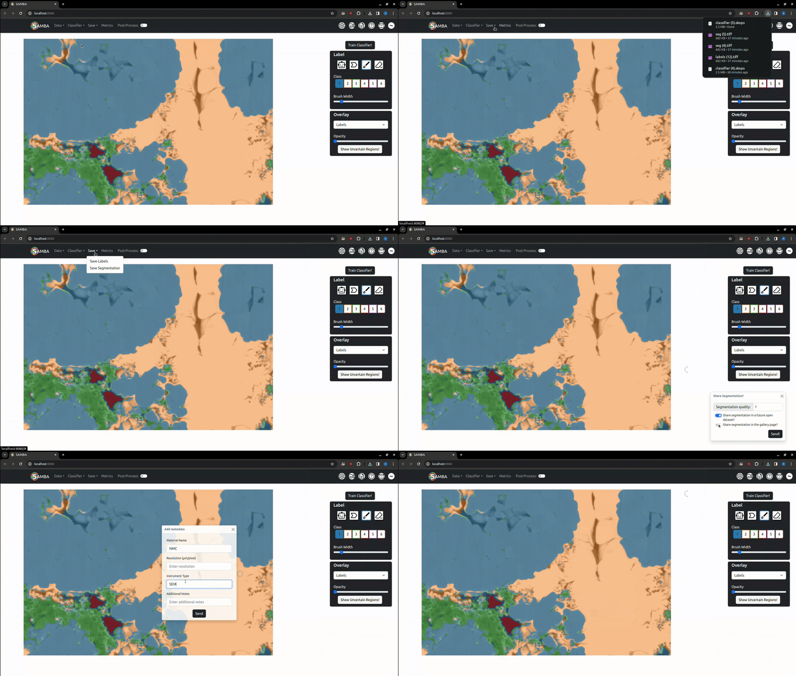
Once a segmentation is saved, a popup will appear asking you to share the segmentation with a future open dataset and/or the gallery page. This is entirely optional - no user data is stored long-term unless explicitly allowed. If shared, another popup will prompt you to add metadata about the image: what material it is, instrument type & resolution and any notes. Once approved, the shared segmentations will be available in the 'Gallery' page.
The added labels will be downloaded. Unlabelled pixels will have a class of 0, this will affect the rescaling relative to the saved segmentation. This option can be useful if you want to use SAMBA as a labelling platform to generate manual labels for training a different segmentation algorithm, like a CNN.
This option in the 'Classifier' tab allows you to download the trained classifier, for use on later datasets either in Python or SAMBA. The available formats are .skops (a secure scikit-learn storage format) and .pkl (a more common format, but unsecure). Note that .pkl classifiers can't be loaded into SAMBA, for security reasons.
When the 'post-process' toggle is active, any labels added (with brush, polygons, smart labels etc.) will edit the saved segmentation, rather than the labels. This can be useful for correcting errors in the segmentation, without needing to re-run the training process.
The gallery page lets you view shared micrographs and their associated segmentations. The toggle switch in the top left lets you view the segmentations. Clicking on a micrograph opens a popup with data descriptions, allowing you to download the data (image, segmentation, labels) associated with that micrograph.
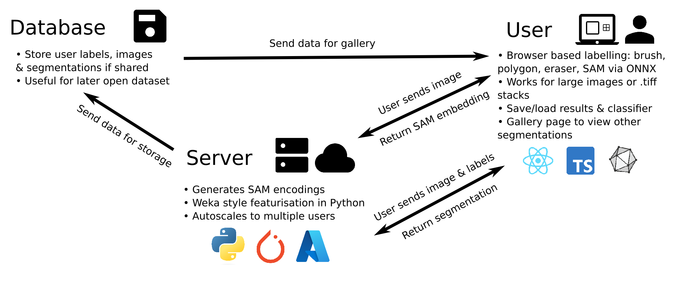
The structure of the web-app is shown above. For local hosting the structure is the same except the server is locally hosted and the database in inaccessible. The structure of the repository is as follows:
frontend contains the React and Typescript code needed to run the labelling app in the browser. It's built using webpack, which compiles the frontend directory before serving it. In this directory there are a few webpack config files in config which don't normally need to be messed with. model contains the .onnx model of the SAM decoder which is needed for client-side smart labelling. src contains the source code that is compiled.
index.tsx is the entrypoint for the application which handles routing between the app and the gallery. App.tsx is the main application: it contains the sub-components that form the GUI, and stores the data needed for labelling (lists of all images, labels, segmentations, etc.). It also handles interfacing with the SAM model and communication with the backend. Functions in app are passed to subcomponents via 'props'. Gallery.tsx contains the code for displaying the gallery (communicating with backend and grid layout).
All the static data files, inlcuding icons, css and the default image with its corresponding SAM encoding.
Contains the sub-components of the GUI. Stage.tsx passes down props (functions) from App.tsx to relevant sub-compenents like the canvas, the navigation bars and the side menu. It also contains code for saving and loading images which it passes to Topbar.tsx to have as onclick events. TIFF loading is achieved using the UTIF.js library. Sidebar.tsx contains user control for labelling, overlays and sub-image navigation (if required). Lots of paramters like brush width, current class are accessed via a large shared context in frontend/src/components/hooks/context.tsx (discussed later). Modals.tsx contains the code for popup windows like settings, feature selection, errors and post-segmentation share prompts. These are conditionally rendered if required.
Canvas.tsx is the most important sub-component - it handles image display and labelling. It is formed of 5 different stacked HTMLCanvas elements. The bottom canvas displays the image, the next segmentations, then labels, then in-progress labels and finally a canvas for animations (like showing a circle at the mouse cursor for the brush or line to a polygon). Once a label is finished, it's ImageData is read from the in-progress label canvas and added to the global label array and then from the label array to the label canvas. The data is transferred from the in-progress canvas by assigning any set pixels in the image of the in-progress canvas the current label class in the label array (assuming the label array is not already set).
The segmentation and label canvases are displayed with their current opacity, which can be changed with the slider. The animated canvas is running a requestAnimationFrame loop to display. All the canvases are React refs, and not States, because we don't want to trigger a re-render when the canvas is changed as it does that automatically (it's a canvas!).
context.tsx and createContext.tsx are the global state of our application, accessible to any component using the AppContext. createContext.tsx can be thought of as the header file for context.tsx, which contains the default values.
These are all functions (not components) to help the app work. canvasUtils.tsx has lots of functions for handling transferring imageData between canvases and accounting for zooms and translations. It also contains the drawing code for drawing in-progress labels to the canvas. Interfaces.tsx is just a list of type declarations for objects - another header file effectively. onnxModelAPI.tsx contains the code to interface with the SAM decoder and scaleHelper.tsx gets images into the right size for SAM .
backend has all the python code for producing SAM embeddings and performing random forest segmentation on a server (local or azure). It also contains code for handling the user data and parameters: for each user a temporary folder is created where featurisations are cached (for speed and to get around RAM limits), segmentaions and labels are stored etc.
Contains 2 functions: one that generates the bytes of the SAM embedding for an input image and another that computes the featurisation of an image via features.py. These features are then saved to the user data directory as compressed numpy files.
Given a set of user selected features and length scales, compute these features for the (sub-)image and return an NxHxW np.array of features. These include 'singlescale' features computed given a length-scale sigma and 'scale-free' features that are computed once.
Deletes and remaps files in user data folder, including deleting all folders older than 2 hours whenever a new user connects.
Contains code to convert user labels and cached featurisations into training data for an sklearn random forest segmentation algorithm. It also includes weighting and sampling code for the training data.
Contains code for segmenting (training and applying random forests) input images by chaining functions in forest_based.py, and also saving for the resulting segmentations and labels as composite tiffs if they are large or a stack.
Simple Flask server that unpacks request arguments before feeding them into the correct function. Note it has some checks that change behaviour depending on if it's running as server or not.
Tests for featurisation and random forest segmentation. Some correctness tests of the filters (i.e is it creating a footprint kernel, what is the shape fo the membrane kernel, etc) followed by comparing the default feature stack of Trainable Weka Segmentation vs SAMBA for a given reference image in test_resoucres/super1.tif. Finally, there is a complete end-to-end test of the segmentations produced by Weka (from an ImageJ installation at $FIJI_PATH) and SAMBA for n=2,3,4 phase micrographs and fixed, rectangular labels defined in the corresponding test_resoucres/n_phase_roi_config.txt . Note you will need to have FIJI installed to run this specific test.
