-
Notifications
You must be signed in to change notification settings - Fork 29
New issue
Have a question about this project? Sign up for a free GitHub account to open an issue and contact its maintainers and the community.
By clicking “Sign up for GitHub”, you agree to our terms of service and privacy statement. We’ll occasionally send you account related emails.
Already on GitHub? Sign in to your account
Equispaced data with gaps vs Non-equispaced data #20
Comments
|
It seems like ndft_adjoint is actually the function to go from signal into frequency space, and ndft to go from frequency into signal space. result: |
|
I am also quite confused about whether nfft_adjoint or nfft correspond to the Fourier transform? which is the inverse Fourier transform. |
|
Depending on what Fourier transform convention you use, the equivalent might be |
|
@jakevdp thank you for your reply! |
|
The formula you quote looks like a standard DFT (both If you have non-uniform data or frequencies, you can use the nfft in this package, and the mathematical form of the forward and adjoint transforms can be seen here: https://github.com/jakevdp/nfft?tab=readme-ov-file#about. You should use the form that most closely matches the quantity you wish to compute. You mention that "the sample interval for time data is change", and I interpret that to mean that you want the output to be on a regular frequency grid, so that suggests the adjoint transform is most appropriate. Additionally, you'll have to correct the output for the difference in phase convention used in the DFT formula you mention. Hope that helps! |
|
Hey we appreciate the response, but as non-mathemeticians it would be super helpful to define the notation. What is obvious to you is not to everyone. You do include many definitions, but could you please also define the hat, f_k, f_j, M, and the word adjoint?
Also it would be great to get feedback on the root of this question - if the behaviour is expected due to theoretical difficulties of non-equispaced data or if I'm just using it wrong.This is a challenging area for self-study.Thanks!William
Yahoo Mail: Search, Organize, Conquer
On Tue, Oct 29, 2024 at 8:03 a.m., Jake ***@***.***> wrote:
The formula you quote looks like a standard DFT (both n and k are on a regular grid) so I would suggest a standard FFT for that case.
If you have non-uniform data, you can use the nfft in this package, and the mathematical form of the forward and adjoint transforms can be seen here: https://github.com/jakevdp/nfft?tab=readme-ov-file#about
Hope that helps!
—
Reply to this email directly, view it on GitHub, or unsubscribe.
You are receiving this because you authored the thread.Message ID: ***@***.***>
|
|
This package provides a fast implementation of two particular summations. Honestly, if the formulas for those summations don’t make sense to you, this might not be the right tool for you to use. |


Can anyone help clear up my misunderstanding?
I used the forward transform to convert a sine wave to frequency domain, then adjoint transform to go back to time domain.
If the data is equispaced, this works well (not pictured).
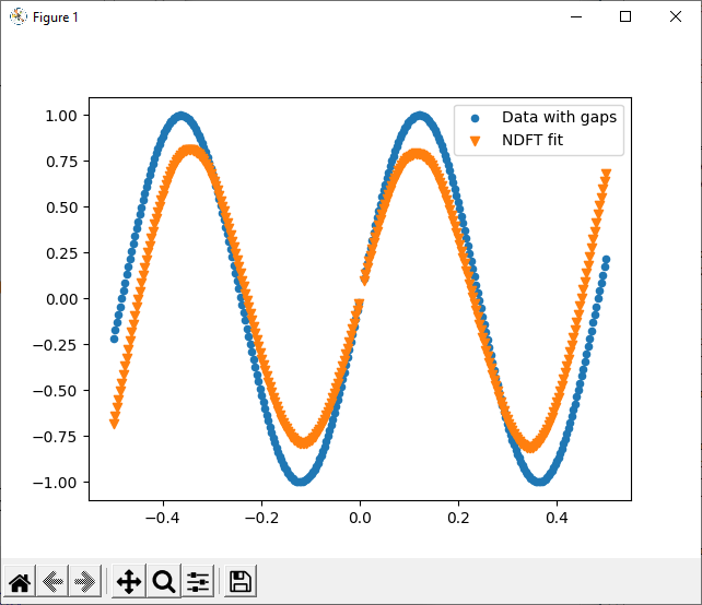
If the data is equispaced but with even a small gap (<1% missing) the reconstruction is smooth, but with incorrect amplitude:

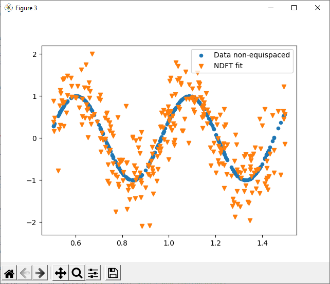
If the data is non-equispaced, the reconstruction is very poor. The Fourier coefficients appear totally random - not an ideal spike, and not spectral leakage.

Is this technique not intended for just these applications? I believe it is and that I've made a mistake.
`import nfft
import numpy as np
import matplotlib.pyplot as plt
freq = 13 #Rad/s
N = 300
x = np.linspace(-0.5, +0.5, N)
f = np.sin(freq*x)
#Equally spaced data with one gap:
gapsize = 2
x=np.delete(x, slice(N//2,N//2+gapsize), axis=0)
f=np.delete(f, slice(N//2,N//2+gapsize), axis=0)
N = len(x)
k = -N//2 + np.arange(N)
f_k = nfft.ndft(x, f)
plt.figure(2)
plt.scatter(k, f_k.real, label="Real")
plt.scatter(k, f_k.imag, label="Imag")
plt.legend()
f_hat = nfft.ndft_adjoint(x, f_k, N)/N
plt.figure(1)
plt.scatter(x, f, s=20, marker='o', label="Data with gaps")
plt.scatter(x, f_hat, s=35, marker='v', label="NDFT fit")
plt.legend()
#Randomly spaced data
x = 0.5 + np.random.rand(N)
f = np.sin(freq*x)
N = len(x)
k = -N//2 + np.arange(N)
f_k = nfft.ndft(x, f)
plt.figure(4)
plt.scatter(k, f_k.real, label="Real")
plt.scatter(k, f_k.imag, label="Imag")
plt.legend()
f_hat = nfft.ndft_adjoint(x, f_k, N)/N
plt.figure(3)
plt.scatter(x, f, s=20, marker='o', label="Data non-equispaced")
plt.scatter(x, f_hat, s=35, marker='v', label="NDFT fit")
plt.legend()
plt.show()
`
The text was updated successfully, but these errors were encountered: