UltraOpt : Distributed Asynchronous Hyperparameter Optimization better than HyperOpt.

---

UltraOpt is a simple and efficient library to minimize expensive and noisy black-box functions, it can be used in many fields, such as HyperParameter Optimization(HPO) and Automatic Machine Learning(AutoML).

After absorbing the advantages of existing optimization libraries such as HyperOpt^[5], SMAC3^[3], scikit-optimize^[4] and HpBandSter^[2], we develop UltraOpt , which implement a new bayesian optimization algorithm : Embedding-Tree-Parzen-Estimator(ETPE), which is better than HyperOpt' TPE algorithm in our experiments. Besides, The optimizer of UltraOpt is redesigned to adapt HyperBand & SuccessiveHalving Evaluation Strategies^[6][7] and MapReduce & Async Communication Conditions. Finally, you can visualize Config Space and optimization process & results by UltraOpt's tool function. Enjoy it !

Other Language: 中文README

• Documentation

  • English Documentation is not available now.

  • 中文文档

• Tutorials

  • English Tutorials is not available now.

  • 中文教程

Table of Contents

• Installation
• Quick Start
  • Using UltraOpt in HPO
  • Using UltraOpt in AutoML
• Our Advantages
  • Advantage One: ETPE optimizer is more competitive
  • Advantage Two: UltraOpt is more adaptable to distributed computing
  • Advantage Three: UltraOpt is more function comlete and user friendly
• Citation
• Referance

Installation

UltraOpt requires Python 3.6 or higher.

You can install the latest release by pip:

pip install ultraopt

You can download the repository and manual installation:

git clone https://github.com/auto-flow/ultraopt.git && cd ultraopt
python setup.py install

Quick Start

Using UltraOpt in HPO

Let's learn what UltraOpt doing with several examples (you can try it on your Jupyter Notebook).

You can learn Basic-Tutorial in here, and HDL's Definition in here.

Before starting a black box optimization task, you need to provide two things:

• parameter domain, or the Config Space
• objective function, accept config (config is sampled from Config Space), return loss

Let's define a Random Forest's HPO Config Space by UltraOpt's HDL (Hyperparameter Description Language):

HDL = {
    "n_estimators": {"_type": "int_quniform","_value": [10, 200, 10], "_default": 100},
    "criterion": {"_type": "choice","_value": ["gini", "entropy"],"_default": "gini"},
    "max_features": {"_type": "choice","_value": ["sqrt","log2"],"_default": "sqrt"},
    "min_samples_split": {"_type": "int_uniform", "_value": [2, 20],"_default": 2},
    "min_samples_leaf": {"_type": "int_uniform", "_value": [1, 20],"_default": 1},
    "bootstrap": {"_type": "choice","_value": [True, False],"_default": True},
    "random_state": 42
}

And then define an objective function:

from sklearn.ensemble import RandomForestClassifier
from sklearn.datasets import load_digits
from sklearn.model_selection import cross_val_score, StratifiedKFold
from ultraopt.hdl import layering_config
X, y = load_digits(return_X_y=True)
cv = StratifiedKFold(5, True, 0)
def evaluate(config: dict) -> float:
    model = RandomForestClassifier(**layering_config(config))
    return 1 - float(cross_val_score(model, X, y, cv=cv).mean())

Now, we can start an optimization process:

from ultraopt import fmin
result = fmin(eval_func=evaluate, config_space=HDL, optimizer="ETPE", n_iterations=30)
result

100%|██████████| 30/30 [00:36<00:00,  1.23s/trial, best loss: 0.023]

+-----------------------------------+
| HyperParameters   | Optimal Value |
+-------------------+---------------+
| bootstrap         | True:bool     |
| criterion         | gini          |
| max_features      | log2          |
| min_samples_leaf  | 1             |
| min_samples_split | 2             |
| n_estimators      | 200           |
+-------------------+---------------+
| Optimal Loss      | 0.0228        |
+-------------------+---------------+
| Num Configs       | 30            |
+-------------------+---------------+

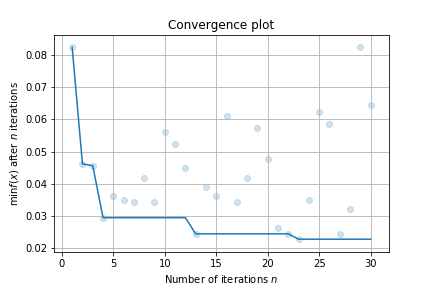
Finally, make a simple visualizaiton:

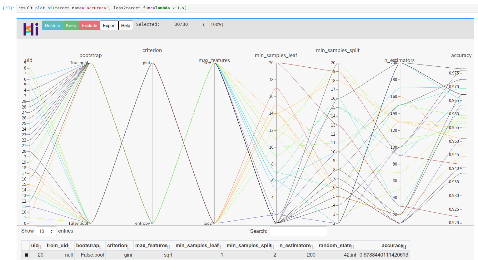
result.plot_convergence()

You can visualize high dimensional interaction by facebook's hiplot:

!pip install hiplot
result.plot_hi(target_name="accuracy", loss2target_func=lambda x:1-x)

Using UltraOpt in AutoML

Let's try a more complex example: solve AutoML's CASH Problem ^[1] (Combination problem of Algorithm Selection and Hyperparameter optimization) by BOHB algorithm^[2] (Combine HyperBand^[6] Evaluation Strategies with UltraOpt's ETPE optimizer) .

You can learn Conditional Parameter and complex HDL's Definition in here, AutoML implementation tutorial in here and Multi-Fidelity Optimization in here.

First of all, let's define a CASH HDL :

HDL = {
    'classifier(choice)':{
        "RandomForestClassifier": {
          "n_estimators": {"_type": "int_quniform","_value": [10, 200, 10], "_default": 100},
          "criterion": {"_type": "choice","_value": ["gini", "entropy"],"_default": "gini"},
          "max_features": {"_type": "choice","_value": ["sqrt","log2"],"_default": "sqrt"},
          "min_samples_split": {"_type": "int_uniform", "_value": [2, 20],"_default": 2},
          "min_samples_leaf": {"_type": "int_uniform", "_value": [1, 20],"_default": 1},
          "bootstrap": {"_type": "choice","_value": [True, False],"_default": True},
          "random_state": 42
        },
        "KNeighborsClassifier": {
          "n_neighbors": {"_type": "int_loguniform", "_value": [1,100],"_default": 3},
          "weights" : {"_type": "choice", "_value": ["uniform", "distance"],"_default": "uniform"},
          "p": {"_type": "choice", "_value": [1, 2],"_default": 2},
        },
    }
}

And then, define a objective function with an additional parameter budget to adapt to HyperBand^[6] evaluation strategy:

from sklearn.neighbors import KNeighborsClassifier
import numpy as np
def evaluate(config: dict, budget: float) -> float:
   layered_dict = layering_config(config)
   AS_HP = layered_dict['classifier'].copy()
   AS, HP = AS_HP.popitem()
   ML_model = eval(AS)(**HP)
   scores = []
   for i, (train_ix, valid_ix) in enumerate(cv.split(X, y)):
       rng = np.random.RandomState(i)
       size = int(train_ix.size * budget)
       train_ix = rng.choice(train_ix, size, replace=False)
       X_train,y_train = X[train_ix, :],y[train_ix]
       X_valid,y_valid = X[valid_ix, :],y[valid_ix]
       ML_model.fit(X_train, y_train)
       scores.append(ML_model.score(X_valid, y_valid))
   score = np.mean(scores)
   return 1 - score

You should instance a multi_fidelity_iter_generator object for the purpose of using HyperBand^[6] Evaluation Strategy :

from ultraopt.multi_fidelity import HyperBandIterGenerator
hb = HyperBandIterGenerator(min_budget=1/4, max_budget=1, eta=2)
hb.get_table()

	iter 0			iter 1		iter 2
	stage 0	stage 1	stage 2	stage 0	stage 1	stage 0
num_config	4	2	1	2	1	3
budget	1/4	1/2	1	1/2	1	1

let's combine HyperBand Evaluation Strategies with UltraOpt's ETPE optimizer , and then start an optimization process:

result = fmin(eval_func=evaluate, config_space=HDL, 
              optimizer="ETPE", # using bayesian optimizer: ETPE
              multi_fidelity_iter_generator=hb, # using HyperBand
              n_jobs=3,         # 3 threads
              n_iterations=20)
result

100%|██████████| 88/88 [00:11<00:00,  7.48trial/s, max budget: 1.0, best loss: 0.012]

+--------------------------------------------------------------------------------------------------------------------------+
| HyperParameters                                     | Optimal Value                                                      |
+-----------------------------------------------------+----------------------+----------------------+----------------------+
| classifier:__choice__                               | KNeighborsClassifier | KNeighborsClassifier | KNeighborsClassifier |
| classifier:KNeighborsClassifier:n_neighbors         | 4                    | 1                    | 3                    |
| classifier:KNeighborsClassifier:p                   | 2:int                | 2:int                | 2:int                |
| classifier:KNeighborsClassifier:weights             | distance             | uniform              | uniform              |
| classifier:RandomForestClassifier:bootstrap         | -                    | -                    | -                    |
| classifier:RandomForestClassifier:criterion         | -                    | -                    | -                    |
| classifier:RandomForestClassifier:max_features      | -                    | -                    | -                    |
| classifier:RandomForestClassifier:min_samples_leaf  | -                    | -                    | -                    |
| classifier:RandomForestClassifier:min_samples_split | -                    | -                    | -                    |
| classifier:RandomForestClassifier:n_estimators      | -                    | -                    | -                    |
| classifier:RandomForestClassifier:random_state      | -                    | -                    | -                    |
+-----------------------------------------------------+----------------------+----------------------+----------------------+
| Budgets                                             | 1/4                  | 1/2                  | 1 (max)              |
+-----------------------------------------------------+----------------------+----------------------+----------------------+
| Optimal Loss                                        | 0.0328               | 0.0178               | 0.0122               |
+-----------------------------------------------------+----------------------+----------------------+----------------------+
| Num Configs                                         | 28                   | 28                   | 32                   |
+-----------------------------------------------------+----------------------+----------------------+----------------------+

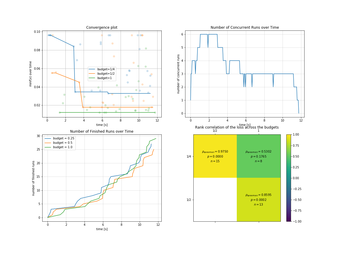
You can visualize optimization process in multi-fidelity scenarios:

import pylab as plt
plt.rcParams['figure.figsize'] = (16, 12)
plt.subplot(2, 2, 1)
result.plot_convergence_over_time();
plt.subplot(2, 2, 2)
result.plot_concurrent_over_time(num_points=200);
plt.subplot(2, 2, 3)
result.plot_finished_over_time();
plt.subplot(2, 2, 4)
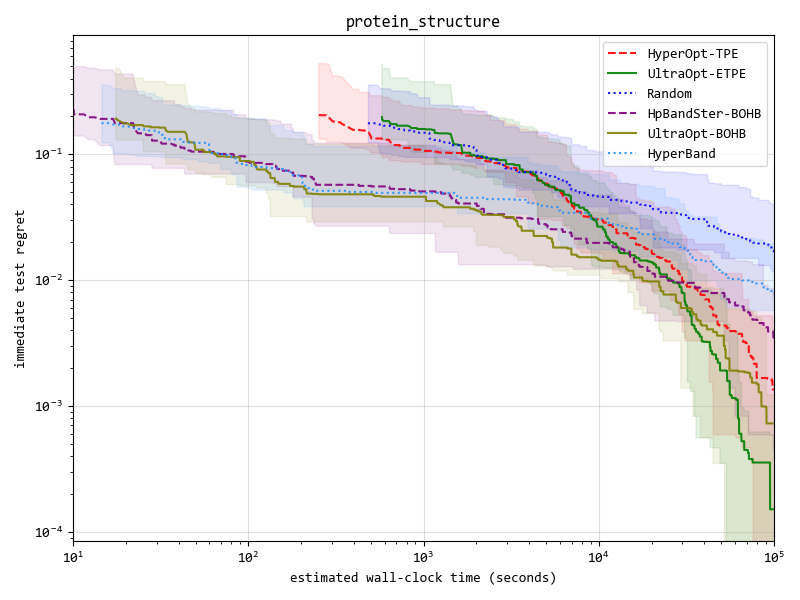
result.plot_correlation_across_budgets();

Our Advantages

Advantage One: ETPE optimizer is more competitive

We implement 4 kinds of optimizers(listed in the table below), and ETPE optimizer is our original creation, which is proved to be better than other TPE based optimizers such as HyperOpt's TPE and HpBandSter's BOHB in our experiments.

Our experimental code is public available in here, experimental documentation can be found in here .

Optimizer	Description
ETPE	Embedding-Tree-Parzen-Estimator, is our original creation, converting high-cardinality categorical variables to low-dimension continuous variables based on TPE algorithm, and some other aspects have also been improved, is proved to be better than HyperOpt's TPE in our experiments.
Forest	Bayesian Optimization based on Random Forest. Surrogate model import scikit-optimize 's skopt.learning.forest model, and integrate Local Search methods in SMAC3
GBRT	Bayesian Optimization based on Gradient Boosting Resgression Tree. Surrogate model import scikit-optimize 's skopt.learning.gbrt model.
Random	Random Search for baseline or dummy model.

Key result figure in experiment (you can see details in experimental documentation ) :

Advantage Two: UltraOpt is more adaptable to distributed computing

You can see this section in the documentation:

• Asynchronous Communication Parallel Strategy

• MapReduce Parallel Strategy

Advantage Three: UltraOpt is more function comlete and user friendly

UltraOpt is more function comlete and user friendly than other optimize library:

	UltraOpt	HyperOpt	Scikit-Optimize	SMAC3	HpBandSter
Simple Usage like fmin function	✓	✓	✓	✓	×
Simple Config Space Definition	✓	✓	✓	×	×
Support Conditional Config Space	✓	✓	×	✓	✓
Support Serializable Config Space	✓	×	×	×	×
Support Visualizing Config Space	✓	✓	×	×	×
Can Analyse Optimization Process & Result	✓	×	✓	×	✓
Distributed in Cluster	✓	✓	×	×	✓
Support HyperBand[6] & SuccessiveHalving[7]	✓	×	×	✓	✓

Citation

@misc{Tang_UltraOpt,
    author       = {Qichun Tang},
    title        = {UltraOpt : Distributed Asynchronous Hyperparameter Optimization better than HyperOpt},
    month        = January,
    year         = 2021,
    doi          = {10.5281/zenodo.4430148},
    version      = {v0.1.0},
    publisher    = {Zenodo},
    url          = {https://doi.org/10.5281/zenodo.4430148}
}

---

Reference

[1] Thornton, Chris et al. “Auto-WEKA: combined selection and hyperparameter optimization of classification algorithms.” Proceedings of the 19th ACM SIGKDD international conference on Knowledge discovery and data mining (2013): n. pag.

[2] Falkner, Stefan et al. “BOHB: Robust and Efficient Hyperparameter Optimization at Scale.” ICML (2018).

[3] Hutter F., Hoos H.H., Leyton-Brown K. (2011) Sequential Model-Based Optimization for General Algorithm Configuration. In: Coello C.A.C. (eds) Learning and Intelligent Optimization. LION 2011. Lecture Notes in Computer Science, vol 6683. Springer, Berlin, Heidelberg.

[4] https://github.com/scikit-optimize/scikit-optimize

[5] James Bergstra, Rémi Bardenet, Yoshua Bengio, and Balázs Kégl. 2011. Algorithms for hyper-parameter optimization. In Proceedings of the 24th International Conference on Neural Information Processing Systems (NIPS'11). Curran Associates Inc., Red Hook, NY, USA, 2546–2554.

[6] Li, L. et al. “Hyperband: A Novel Bandit-Based Approach to Hyperparameter Optimization.” J. Mach. Learn. Res. 18 (2017): 185:1-185:52.

[7] Jamieson, K. and Ameet Talwalkar. “Non-stochastic Best Arm Identification and Hyperparameter Optimization.” AISTATS (2016).