-
Notifications
You must be signed in to change notification settings - Fork 331
Association location algorithm of SPL
When associating the big data tables, conditional filtering is sometimes performed on the associated tables first. For the case where the associated fields are the primary keys or part of primary keys, SPL provides the association location algorithm on the basis of the ordered merge association algorithm (refer to: )to improve the computing performance of the association after filtering.
Let's first look at the case where the associated tables are joined by all primary keys (we call such tables are the homo-dimension table from each other). Assuming that there are two large tables, table a and table b, and they are already stored in order by the primary key id in advance, the association relationship between them is as shown in Figure 1 below:

Figure 1 Tables a and b
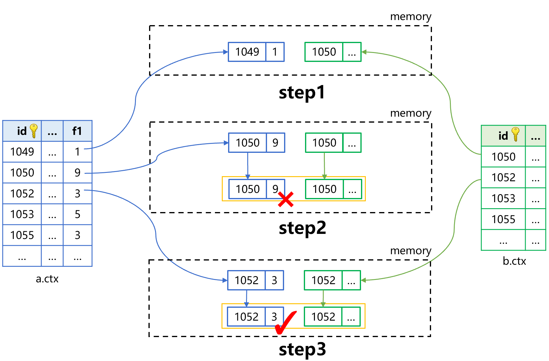
Now, we want to join these two tables by id, and filter out the records whose f1 is 3. A simple method is to associate them by the primary key and then filter. See Figure 2 for the general process:

Figure 2 Associating first and then filtering
In Figure 2, first, take out the records in order from tables a and b to do association, and then judge whether f1 is 3. If it is 3, output the result, if not, discard it. In this way, each table will be traversed once, and it will be very time-consuming when the table is large.
If the records that meet the condition after filtering still account for the vast majority, it is necessary to traverse both tables. But if there are only a few records left after table a is filtered, it is unnecessary to traverse the whole table b. The traversal of one large table can be avoided if using the ordered characteristics of associated fields to find the corresponding data in table b based on the filtered data of table a.
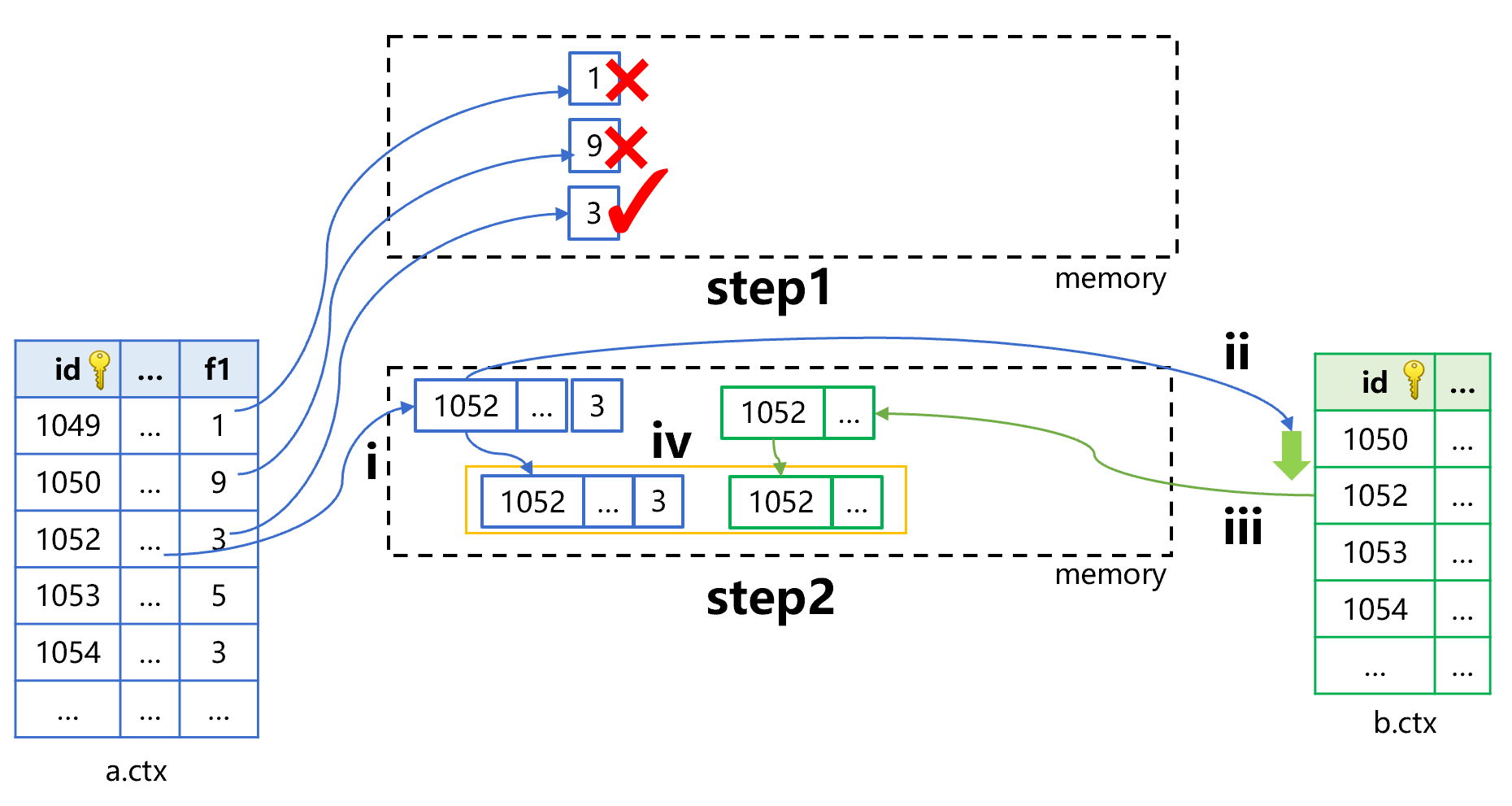
This method is the association location algorithm provided by SPL, and the process of performing the above calculation requirements is roughly as shown in Figure 3 below:

Figure 3: Association location algorithm (step 1 and 2)
In this figure, step1 uses the pre-cursor filtering technology (refer to: Performance Optimization - 4.1 [Traversal technology] Cursor filtering) to read one field f1 of only one record from table a to judge whether it is 3. If it is not 3, discard it and take the next record of table a, and if it is, perform step2.
step2 is relatively complicated, we divide it into four small steps. Step i is to continue reading other fields of table a except f1; Step ii is to search for the primary key in table b using the value 1052 of the primary key id of table a; Steps iii and iv are to find the records in table b, and then generate a new associated record with the records in table a.
Compared with figure 2, for the records at f1 field in table a that do not meet the condition, there is no need to read other fields. For example: for the two records whose id is 1049 and 1050, it saves time to read other fields. Meanwhile, there is no need to read the whole record whose id is 1050 in table b. Overall, the smaller the result set in table a that meets the filtering condition, the lager the amount of read reduced and the more obvious the performance improvement effect.
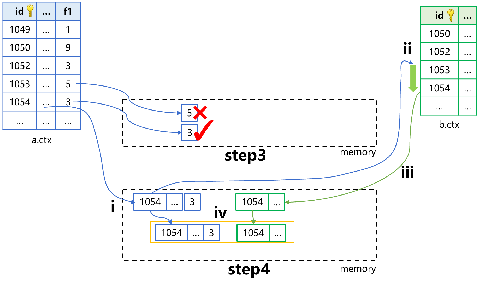
Continue to perform steps 3 and 4 of the association location calculation, roughly as shown in Figure 4 below:

Figure 4: Association location algorithm (step 3 and 4)
Step 3 is to continue using the pre-cursor filtering technology to search for the record whose f1 is 3. After finding the record, perform step4.
Step4 is also divided into four small steps. Let’s focus on step ii since other small steps are the same as those in step2: use the value of the primary key id, i.e., 1054 to do the primary key search in table b. In this search, it only needs to continue to search forward from the last position point (id value is 1052), and there is no need to search from the beginning of table b.
As can be seen from Figures 3 and 4, since the primary key id of the records taken out from table a is ordered, the records taken from table b by id will not be repeated. Moreover, the reading process is to scan table b from front to back, the worst case is to traverse table b only once, and there will be no repeated traversal.
If the result set left is small after the table a is filtered, the association location algorithm can greatly decrease the amount of data read from the hard disk, and can also avoid traversing the whole table b, and hence a better performance can be obtained.
However, it’s not easy to implement the association location algorithm, and the its code is more complicated. Moreover, the cost of this algorithm itself is not low, which may offset the advantage of smaller reading amount. For the specific application scenario, testing is necessary.
SPL encapsulates this algorithm, and it needs to use the new() function to perform the association location of homo-dimension tables. The SPL code is roughly as follows:
| A | |
|---|---|
| 1 | =file("a.ctx").open().cursor(id,f1,…;f1==3) |
| 2 | =file("b.ctx").open().new(A1,f1,…) |
| 3 | =A1.fetch(1000) |
A1 defines the pre-cursor filter calculation for table a. In order to perform subsequent primary key search in table b, the primary key id of table a need to be taken out here.
A2 adopts the association location algorithm, using the filtered records of table a to fetch the records of table b. The delayed cursor is defined here, and no real calculation occurs.
A3 fetches the data from the delayed cursor formed in A2, which can also be used to do other operations.
The new function in A2 is associated by the primary key, and does not specify the associated field when used. When SPL finds that the primary key of table a has only one id field, it will use the first field in table b to correspond to it. Generally, since the homo-dimension tables have the same number of primary key fields, when the primary keys of both tables a and b have n fields, SPL will correspond them one by one in order. The name of the field does not affect the correspondence of the primary key fields.
The new function is to use the primary key of table a to search in table b, therefore, the search result is based on the records of table b to add the fields of table a, which means the primary key that exists in the table a but does not exist in table b, the corresponding record will not appear in the result.
When the primary key of one table associates with part of primary keys of other tables, we call it the primary-sub table association. The first table is called the primary table and other tables are sub-tables. Let's take a look at the case where the association location calculation is made between a primary table and a sub table.
For example, the relationship between the order table and the detail table is shown in Figure 5:

Figure 5: Relationship between order table and detail table
What we want to do is to associate the two tables and filter the order table by the condition cid==10096, and then group by odate, and finally sum the price*quantity.
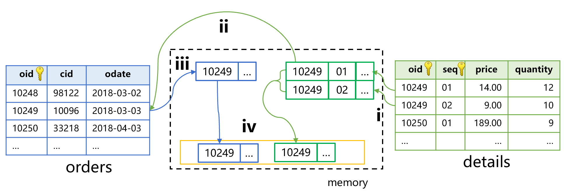
The difference from Figures 3 and 4 is that we use the filtered order data to search for part of the primary keys in the detail table rather than all primary keys. The search may get a result set of multiple records. See Figure 6 below for the general process:

Figure 6 Filtering order table (primary table) by condition
Step i is to read the order table in order to find one record that meets the condition, and use the oid value 10249 of its the primary key to search the first field of the detail table.
Step ii, find two records. In step iii, the search object is the detail table, and what is returned is the records of the detail table. Therefore, the result is based on the detail table, and two new associated records will be generated, which means, one record of the order table needs to be repeated twice.
In SPL, when the primary table (order table) associates with the sub-table after being filtered by condition, the news() function needs to be used. The code is roughly as follows:
| A | |
|---|---|
| 1 | =file("orders.ctx").open().cursor(oid,odate;cid==10096) |
| 2 | =file("details.ctx").open().news(A1,odate,price,quantity) |
| 3 | =A2.groups(dt;sum(price*quantity)) |
A1 defines the pre-cursor filter calculation for the order table. In order to perform subsequent search in the detail table, the primary key oid needs to be taken out here.
In A2, use the results filtered in A1 to search in the detail table. Using each oid in the order table (primary table) that meets the condition to search the detail table (sub-table) may obtain multiple records. The news function used here indicates that the fields of primary table will be copied according to the number of the records of associated sub-table to form a multi-row result set.
The news function in A2 also does not specify the associated field. When SPL finds the primary key in A1 (primary table) has only one field oid, it will use the first field oid in detail table (sub table) to correspond to it. Generally, for the primary-sub table association, the number of primary key fields of primary table is definitely less than that of sub-table. When the primary key of primary table consists of n fields, SPL will find the first n fields corresponding to them in the detail table (sub-table) according to the order of fields.
If the condition to be filtered is quantity>10 in the detail table, the calculation process will roughly become as shown in Figure 7 below:

Figure 7 Filtering detail table (sub table) first
Step i, traverse the detail table by the filter condition. First find two records that meet the condition, and whose oid are all 10249, and seq are 1 and 2 respectively. Step ii, use the oid value 10249 to search the order table, and get one record. In step iii, the search object of the primary key is the order table, and the returned result is the records of order table. Therefore, the result is based on the order table. We need to aggregate the two records in the detail table, and then generate a new associated record with the record in order table.
Filtering of detail table (sub-table) first followed by association of primary table implemented by SPL also uses the new function. The code is roughly as follows:
| A | |
|---|---|
| 1 | =file("details.ctx").open().cursor(oid,price,quantity;quanity>10) |
| 2 | =file("orders.ctx").open().new@z(A1,odate,sum(price*quantity):amount) |
| 3 | =A2.groups(odate;sum(amount)) |
A1 defines the pre-cursor filter calculation for the detail table. In order to perform subsequent primary key search of order table, the oid field needs to be taken out here.
In A2, the new function is to use the results filtered in A1 to search the order table. The result of new is the records of order table, and it should be based on the records of order table. Moreover, one oid of the detail table that meets the condition may correspond to multiple records. Therefore, when using the new function here, it needs to first perform an aggregation on A1.
Why adding @Z option to new here?
As mentioned earlier, by default, the new function will see how many primary keys A1 has, and then use the first few fields in the order table to correspond to such primary keys. However, the cursor in A1 only takes part of the primary keys, i.e., oid, and does not take the second primary key seq, therefore, the result cursor calculated in A1 loses the primary key. In this case, the primary key field of A1 cannot be used to correspond to the first few fields of the order table.
@z means that the new function inversely uses the primary key of the order table to find the corresponding number of fields in A1 for correspondence.
SPL Resource: SPL Official Website | SPL Blog | Download esProc SPL | SPL Source Code